ARIMA Diagnostics in R: checkresiduals() and Ljung-Box
ARIMA diagnostics check whether a fitted model's leftovers, called residuals, are white noise: pure randomness with no pattern left to forecast. In R, one function, checkresiduals(), draws a time plot, an autocorrelation plot, and a histogram of those residuals and runs the Ljung-Box test, all in a single call. A Ljung-Box p-value above 0.05 means the residuals pass. This tutorial uses base R plus the forecast package.
What are ARIMA residuals, and why must they be white noise?
A residual is the gap between what actually happened and what your model predicted for that same point in time. Fit an ARIMA model, ask it to predict each observation one step ahead, subtract the prediction from the truth, and the pile of errors you are left with are the residuals. If those errors still trend, cycle, or repeat every twelve months, the model missed real structure that you could have forecast. A trustworthy model leaves residuals with no usable pattern at all.
That "no usable pattern" idea has a precise name: white noise. A white noise series has four traits, and every ARIMA diagnostic is really just a test for one of them.
- Zero mean. The errors are not consistently high or low, so the model is not biased.
- Constant variance. The spread of the errors stays steady over time, not calm early and wild later.
- No autocorrelation. Today's error tells you nothing about tomorrow's error.
- Roughly normal. The errors form a bell shape. This one is a bonus: it is needed for honest prediction intervals, not for the point forecast.
Let's make this concrete. We will fit an ARIMA model to WWWusage, a built-in series of 100 minute-by-minute readings of users connected to a web server. The auto.arima() function from the forecast package searches candidate models and returns the best one, so we can focus on the diagnostics rather than the model hunt.
The printout tells us auto.arima() picked an ARIMA(1,1,1): one autoregressive term, one difference, and one moving-average term. The ar1 and ma1 rows are the estimated coefficients, and sigma^2 is the variance of the residuals. This is the model whose residuals we are about to inspect. The coefficients look fine, but coefficients alone never tell you whether the model is good enough. Only the residuals can do that.
Try it: Pull the residuals out of fit_good with residuals() and check the first two white-noise traits: is their mean near zero and is their variance stable? Store the residuals in ex_res and report the mean and variance.
Click to reveal solution
Explanation: The mean, 0.3036, sits close to zero relative to the residual spread, and the variance, 9.7, is roughly the sigma^2 the model reported. Those are the first two boxes ticked. checkresiduals() will check the other two for us next.
How do you run checkresiduals() in one line?
Checking each white-noise trait by hand would be tedious, so the forecast package bundles all of them into a single function. Pass a fitted model to checkresiduals() and it produces three diagnostic plots and prints a formal test of autocorrelation. It is the fastest honest answer to "is my model good enough?"
Two things happen at once. A three-panel figure appears (we read it in the next section), and the text above is printed to the console. That text is the Ljung-Box test, the numerical verdict on whether the residuals still carry autocorrelation. The line that matters most is the p-value: 0.4499. Because it is comfortably above 0.05, the test finds no evidence of leftover autocorrelation, so the residuals behave like white noise and the model passes.
The Model df: 2 and Total lags used: 10 lines explain how the test was set up, and we unpack them when we reach the Ljung-Box section. For now, read the p-value first: high is good.
Try it: Sometimes you want the test result without redrawing the plots, for example inside a loop that fits many models. Ask checkresiduals() for the numbers only by setting plot = FALSE.
Click to reveal solution
Explanation: With plot = FALSE you get the exact same Ljung-Box test, just without the figure. This is handy when you are comparing dozens of models and only care about which ones pass.
How do you read the three residual plots?
The figure checkresiduals() draws is where you catch problems the single p-value can hide. It stacks three views of the same residuals, and each one checks a different white-noise trait. Here is the figure for our passing model.

Figure 1: The output of checkresiduals() for a model that passes. Flat residuals, ACF spikes inside the bands, and a roughly normal histogram.
Read the panels like this:
- Top: the residuals over time. You want a formless cloud bouncing around zero with a steady width. Our top panel does exactly that, which supports the zero-mean and constant-variance traits. A funnel that widens to the right would signal changing variance.
- Bottom left: the ACF, or autocorrelation function. Each bar shows how strongly the residuals correlate with themselves a fixed number of steps (lags) apart. The two dashed blue lines are the "just noise" band, drawn at plus and minus $1.96/\sqrt{n}$. Bars inside the band are indistinguishable from zero. Every bar here sits inside the band, so there is no autocorrelation to worry about.
- Bottom right: the histogram. The bars are the residual distribution and the orange curve is a matched normal. A close match means prediction intervals will be trustworthy. Ours is roughly bell-shaped.
The ACF band is the workhorse, so let's compute it rather than eyeball it. With 100 observations, the band sits at $1.96/\sqrt{100} = 0.196$. We can count how many of the first ten autocorrelations poke outside it.
We stored the residuals in res, computed the band width, and then pulled the autocorrelations straight from acf(), dropping the lag-0 value (which is always 1) with [-1]. The final line counts how many exceed the band. The answer is 0, which matches what the eye saw in Figure 1: every spike is inside the lines.
Try it: Ten lags is the default, but longer series can hide autocorrelation further out. Re-count the exceedances using the first 20 lags instead. Use ex_band and ex_acf so you do not overwrite res.
Click to reveal solution
Explanation: Even out to 20 lags, zero autocorrelations break the band. The residuals are clean at both short and long horizons, which is exactly what a white-noise series should look like.
What is the Ljung-Box test and how do you read its p-value?
Eyeballing an ACF is fine for one model, but you need a single objective number when you compare models or automate the check. That number is the Ljung-Box test. Instead of judging each lag separately, it asks one combined question: taken together, are the first several autocorrelations all close enough to zero to be pure chance? Because it pools many lags into one statistic, it is called a portmanteau test.
The test is a hypothesis test, so it starts from a null hypothesis and tries to reject it.
- Null hypothesis: the residuals are white noise (no autocorrelation up to lag $h$).
- A large p-value (above 0.05) means you cannot reject the null, so the residuals look like white noise. This is the outcome you want.
- A small p-value (0.05 or below) means you reject the null, so autocorrelation remains and the model needs work.
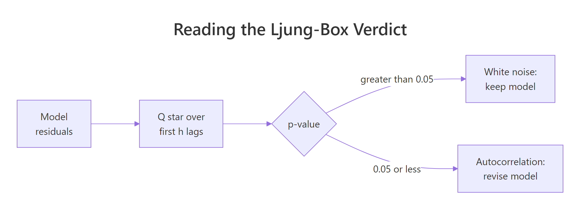
Figure 2: How to turn a Ljung-Box p-value into a keep-or-revise decision.
Notice the logic runs opposite to most tests you have seen: here a small p-value is bad news. That is because the null you are hoping to keep is the good outcome. If you want the formula behind the statistic, here it is. If not, skip to the next section, the code is all you need.
The test squares each autocorrelation, weights it, and adds the pieces up into a single statistic $Q^*$:
$$Q^* = n(n+2) \sum_{k=1}^{h} \frac{\hat{\rho}_k^{2}}{n-k}$$
Where:
- $n$ = the number of residuals
- $h$ = how many lags you test (labelled "Total lags used" in the output)
- $\hat{\rho}_k$ = the residual autocorrelation at lag $k$
- $Q^*$ = the pooled statistic, compared against a chi-squared distribution to get the p-value
The one subtlety is the degrees of freedom. You did not know the true model, you estimated it, and each estimated ARIMA term uses up a little of the data's freedom to wiggle. So the test subtracts the number of fitted terms from the lag count: $df = h - (p + q)$. In our WWWusage model that is $10 - 2 = 8$, which is the df = 8 the output showed. That is also why the output printed Model df: 2: it is reminding you it already subtracted the two ARIMA coefficients.
To see the test behave, let's run it on a series we know is white noise, because we generate it from scratch with rnorm().
We drew 120 independent normal values, which are white noise by construction, and tested them. The p-value, 0.4008, is well above 0.05, so the test correctly declines to reject the null. This is the behaviour you want to see from residuals of a good model.
df equals the full 10 lags. When you test model residuals by hand, you must set that adjustment yourself, which is the next section.Try it: Now run the test on a series that is obviously not white noise: the raw AirPassengers data, which trends upward and repeats every year. Predict the p-value before you run it.
Click to reveal solution
Explanation: The statistic is very large and the p-value is essentially zero, so the test firmly rejects white noise. A raw seasonal, trending series carries strong autocorrelation at many lags, which is exactly the structure a good ARIMA model is supposed to remove from the residuals.
How do you run the Ljung-Box test yourself with Box.test()?
checkresiduals() is the convenient front door, but under the hood it calls base R's Box.test(). Running Box.test() directly is useful when you want to choose your own lag, when you are not using forecast package objects, or when you simply want to understand what the wrapper is doing. The catch is that you have to supply the degrees-of-freedom adjustment yourself, through the fitdf argument.
Our WWWusage model is an ARIMA(1,1,1), so $p + q = 1 + 1 = 2$. We pass fitdf = 2 to tell the test that two coefficients were estimated. Let's confirm it reproduces the checkresiduals() output exactly.
The statistic 7.8338 and the p-value 0.4499 are identical to what checkresiduals() reported earlier. The one cosmetic difference is that Box.test() labels the statistic X-squared while checkresiduals() labels it Q*; they are the same number. Two rules make Box.test() match the wrapper:
- Lag. The wrapper's default is 10 lags for a non-seasonal series and twice the seasonal period for a seasonal one. We passed
lag = 10to match. - fitdf. Set it to the number of AR and MA terms, that is $p + q$ (plus seasonal $P + Q$ if present). Do not count the mean, drift, or intercept: those are not autoregressive or moving-average terms.
fitdf and lag correctly on its own, which removes the most common source of a wrong p-value.Try it: See what happens when you forget the adjustment. Rerun the test on fit_good with fitdf = 0 and compare the df and p-value to the correct version above.
Click to reveal solution
Explanation: The statistic is unchanged, but df is now 10 instead of 8, and the p-value drifts to 0.6451. Forgetting fitdf makes the test too lenient, so a shaky model can slip through. The statistic stays the same; only the yardstick you compare it against moves.
What should you do when a diagnostic fails?
A failing diagnostic is a to-do list, not a dead end. The residual plots tell you which white-noise trait broke, and each broken trait points to a specific fix. Let's manufacture a failure on purpose. AirPassengers has a strong yearly cycle, so if we fit a non-seasonal model with Arima(), it cannot capture the seasonality and the leftover pattern will show up in the residuals.
The p-value is essentially zero, a decisive fail. The residuals still hold autocorrelation, which means real structure escaped the model. The plot shows exactly where.

Figure 3: A failing diagnostic. The ACF shows tall spikes at the seasonal lags, so the model missed the yearly cycle.
Look at the ACF panel: the bars at lag 12 and lag 24 rise far outside the band. Because the data is monthly, spikes at multiples of 12 mean the residuals still repeat every year. The model never learned the season. The fix is to add seasonal terms and, because the yearly swings in AirPassengers grow over time, to stabilise the variance with a log transform (lambda = 0).
The p-value jumps from near zero to 0.233. By adding a seasonal moving-average term and a seasonal difference, and by taming the growing variance with the log transform, the residuals now pass. The seasonal spikes are gone. This is the whole loop in miniature: read the failure, change the matching part of the model, re-check.
Figure 4 maps the most common failures to their fixes.
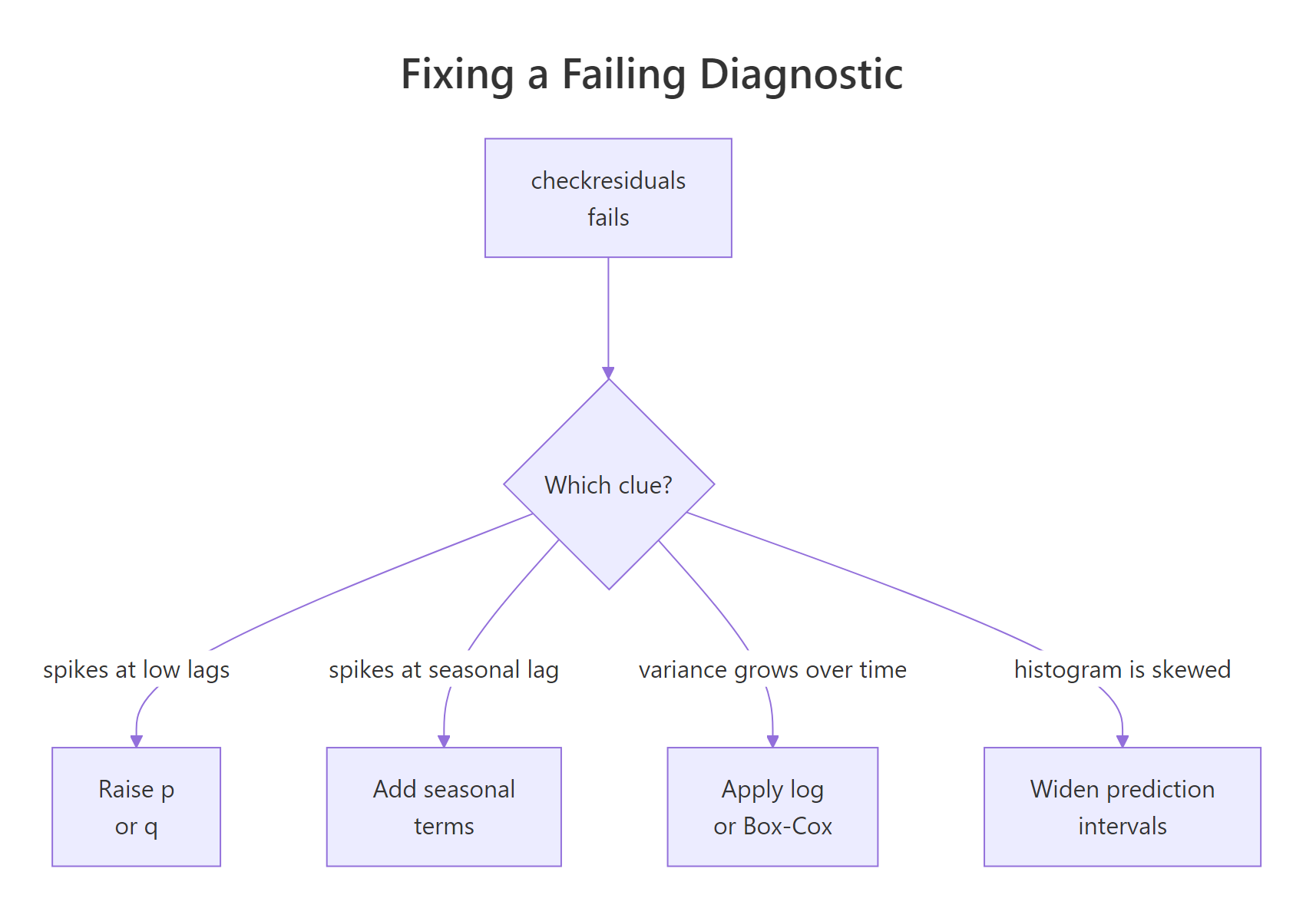
Figure 4: Which model change to try for each kind of diagnostic failure.
Try it: Confirm the repaired model really passes by printing just its Ljung-Box result.
Click to reveal solution
Explanation: The p-value of 0.233 clears the 0.05 bar, so the seasonal model's residuals are white noise. The fix worked, and you can trust this model's forecasts.
Complete Example: diagnose an ARIMA model end to end
Let's put every step together on a fresh series. USAccDeaths records monthly accidental deaths in the United States and has a clear yearly cycle. We will fit a model, diagnose it, and forecast only after it passes.
First, fit the model with auto.arima() and read what it chose.
The search landed on a seasonal model, ARIMA(0,1,1)(0,1,1)[12], which already accounts for the yearly pattern. Before we trust it, we diagnose the residuals.
The p-value is 0.336, so the residuals pass the Ljung-Box test and the accompanying plots (which you will see when you run this) show no leftover pattern. The model has captured the structure in the series. Now, and only now, is it safe to forecast.
Each row is a future month with a point forecast and 80% and 95% prediction intervals. Those intervals are only believable because the residuals passed the diagnostics first. Diagnose, then forecast, in that order, every time.
Practice Exercises
These exercises combine the steps above. Use distinct variable names so you do not overwrite the tutorial's objects.
Exercise 1: Fit and diagnose a new model
Fit an ARIMA model to the built-in lh series (48 readings of a luteinizing hormone level) with auto.arima(), run checkresiduals(), and decide whether the residuals pass. State the p-value and your verdict.
Click to reveal solution
Explanation: auto.arima() chose an ARIMA(1,0,0) with a non-zero mean. The Ljung-Box p-value of 0.405 is above 0.05, so the residuals are white noise and the model passes.
Exercise 2: Match the p-value with Box.test()
Reproduce the exact Ljung-Box p-value from Exercise 1 using Box.test() on residuals(lh_fit). The trap: the model has a mean term. Work out the correct fitdf so your df matches the 9 that checkresiduals() reported.
Click to reveal solution
Explanation: The model is ARIMA(1,0,0), so $p + q = 1$: only the single AR term counts. The mean is not an AR or MA term, so it is excluded from fitdf. Passing fitdf = 1 gives df = 10 - 1 = 9 and the p-value 0.405, matching checkresiduals() exactly. If you had counted the mean and used fitdf = 2, the df would drop to 8 and the p-value would change.
Exercise 3: Repair a failing model
The fit_bad model from earlier failed its diagnostics on AirPassengers. Build a repaired model, store it in my_fix, and show that its Ljung-Box test now passes. Let auto.arima() do the work, but stabilise the variance with a log transform.
Click to reveal solution
Explanation: Setting lambda = 0 applies a log transform, and auto.arima() then finds a seasonal model on its own. The Ljung-Box p-value of 0.233 clears 0.05, so the repaired model passes where fit_bad failed.
Frequently Asked Questions
What counts as a good p-value for the Ljung-Box test?
Any p-value above 0.05 passes: it means the test cannot reject the null that the residuals are white noise, so no leftover autocorrelation was found. Read it the opposite way round to most tests, where a small p-value is the interesting result. A high p-value is not a score of overall model quality, only a sign that this one test found no autocorrelation.
Why does checkresiduals() report a different p-value than Box.test()?
checkresiduals() subtracts your model's estimated terms through the degrees-of-freedom adjustment and picks the lag for you, while a bare Box.test() does neither. If you call Box.test() with fitdf = 0, the df is too high and the p-value comes out larger. Set fitdf to the number of AR and MA terms ($p + q$, plus seasonal $P + Q$) and use the same lag, and the two match exactly.
How many lags should I test?
checkresiduals() uses 10 lags for a non-seasonal model and twice the seasonal period for a seasonal one, and those defaults are sensible starting points. Testing too few lags can miss autocorrelation that sits further out; testing too many spreads the statistic thin and weakens the test. When in doubt, let checkresiduals() choose.
My residuals pass Ljung-Box but the forecasts still look off. Why?
The Ljung-Box test only looks for autocorrelation. It says nothing about changing variance or a wrong transform, and either of those can pass the test yet make the prediction intervals too narrow or too wide. Always read the residual time plot for a funnel shape and the histogram for skew, not just the p-value.
Do I count the intercept, mean, or drift in fitdf?
No. fitdf counts only the autoregressive and moving-average terms, that is $p + q$ (and seasonal $P + Q$ if present). A mean, drift, or intercept term is not an AR or MA term, so it is excluded, which is the trap in Exercise 2 above.
Summary
ARIMA diagnostics come down to one question asked four ways: are the residuals white noise? Here is the whole workflow at a glance.
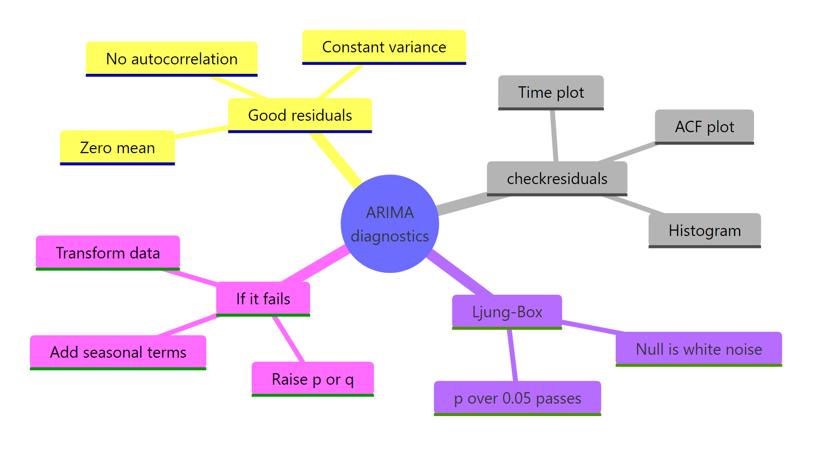
Figure 5: The full ARIMA diagnostics workflow at a glance.
The key takeaways:
| Check | Tool | Pass looks like |
|---|---|---|
| No autocorrelation | ACF panel, Ljung-Box test | Spikes inside the bands; p-value above 0.05 |
| Zero mean and steady variance | Residual time plot | A flat, even-width cloud around zero |
| Normal errors | Histogram panel | Bars matching the overlaid normal curve |
| Reproduce the test by hand | Box.test(..., fitdf = p + q) |
Same statistic and p-value as the wrapper |
Three rules to carry forward. First, read the Ljung-Box p-value the opposite way to most tests: high means the model is good. Second, when you call Box.test() yourself, set fitdf to the count of AR and MA terms, never the mean or drift. Third, always diagnose before you forecast, because a prediction interval is only honest if the residuals that produced it are white noise.
References
- Hyndman, R.J., & Athanasopoulos, G. - Forecasting: Principles and Practice, 3rd Edition. Section 3.3, Residual diagnostics. Link
- Hyndman, R.J., & Athanasopoulos, G. - Forecasting: Principles and Practice, 3rd Edition. Section 9.7, ARIMA modelling in R. Link
- forecast package -
checkresiduals()reference. Link - R Core Team -
Box.test()documentation (stats package). Link - Ljung, G.M., & Box, G.E.P. - "On a measure of lack of fit in time series models." Biometrika 65(2), 297-303 (1978). Link
- R Core Team - An Introduction to R. Link
Continue Learning
- ARIMA in R: build ARIMA models from the ground up, the step before you diagnose them.
- How to Choose ARIMA Order in R: pick the p, d, and q values that give you white-noise residuals in the first place.
- ETS vs ARIMA in R: compare ARIMA with exponential smoothing and learn when each one wins.