Sub-Daily Forecasting in R: the Multiple-Seasonality Playbook
Sub-daily data, meaning anything recorded hourly, half-hourly or every few minutes, usually repeats on more than one cycle at once: one shape that repeats every day, and a different shape that repeats every week. A standard seasonal model can only hold one of those cycles. The playbook is to name every period your data actually has, hand them all to a model that accepts more than one, and score the candidates on a holdout before you trust any of them.
Why does one seasonal period fail on sub-daily data?
The taylor dataset that ships with the forecast package is half-hourly electricity demand for England and Wales, twelve complete weeks of it. Demand has an obvious daily rhythm: low overnight, high in the evening. It also has a second rhythm that is easy to miss entirely. Average each day of the week separately and it jumps straight out at you.
Walking through the code: each day holds 48 half-hourly readings, so rep(day_names, each = 48, times = 12) stamps a weekday label onto every one of the 4032 observations, and tapply() then averages the demand within each label.
Now read the numbers. Thursday averages 31402 megawatts and Sunday averages 25233. That is a gap of over 6000 megawatts, roughly a fifth of total demand, and it has nothing to do with the time of day. It is purely about which day of the week it is. Weekdays look like each other and weekends look like each other, and the two groups are not close.
So this series repeats on two clocks at the same time. Before going further, it helps to know exactly how much data we are holding.
Twelve clean weeks, 84 days, 4032 readings. That divides evenly, which will matter shortly.
Here is the crucial idea, and it is the one thing that trips up almost everybody moving from monthly data to sub-daily data. In R, a seasonal period is a count of observations, not a length of time. Monthly data has period 12 because twelve rows make a year. Half-hourly data has period 48 because 48 rows make a day. But 336 rows make a week, and that is a perfectly real cycle too. A plain ts object stores one number for frequency, so it can hold 48 or it can hold 336. It cannot hold both.
Let us find out what that costs. We will hold back the final two days and forecast them. Because the series starts on a Monday and runs a whole number of weeks, the last two days are exactly Saturday and Sunday, which is the hardest pair for a model that has never heard of weekends.
The simplest possible forecast is the seasonal naive: predict each future point using the matching point one full cycle ago. With a period of 48, "one cycle ago" means yesterday.
One new function appears in the block below. msts() is the multi-seasonal cousin of ts: it stores a whole vector of seasonal periods instead of a single number. The next section takes it apart properly, so for now just read seasonal.periods = 48 as "one cycle is 48 rows" and seasonal.periods = c(48, 336) as "there are two cycles, one of 48 rows and one of 336".
The code holds out the last 96 readings as test, builds two versions of the training data, and scores the period-48 forecast against the holdout. accuracy() returns a two-row matrix, training set then test set, so [2, ] picks the test-set row, which is the one that counts.
Three error measures come back. RMSE and MAE are both average error sizes in megawatts, with RMSE weighting the large misses more heavily. MAPE is that same error written as a percentage of actual demand, which makes it the easiest of the three to read when you do not have the scale of the series in your head.
A MAPE of 19.02 means the forecast is off by about 19 percent on average. That is a bad forecast for a series this regular. The model is repeating Thursday and Friday onto Saturday and Sunday, and weekends simply do not look like weekdays.
Now change one thing. Keep the same data, the same method, the same holdout, and only tell R that a week is also a cycle.
The error falls from 19.02 percent to 1.74 percent. That is roughly eleven times more accurate, from a change that involved no new model, no tuning and no extra data. All that happened is that snaive() now repeats last Saturday onto this Saturday instead of repeating last Thursday onto it.
Try it: The day-of-week averages showed the weekly cycle. Now measure the daily one. Compute the average demand at each half-hour of the day, then report the peak, the trough, and the percentage gap between them.
Click to reveal solution
Explanation: The daily swing is 61.6 percent from trough to peak, which is much larger than the weekly swing of about 20 percent. Both are real, and a good model needs both. The daily cycle is the loud one, which is exactly why the weekly one is so easy to overlook.
How do you find which seasonal periods your data actually has?
You do not have to guess. There are two steps, and doing both is what separates a reliable answer from a hopeful one. First derive the candidate periods by arithmetic from your sampling interval, then confirm each candidate against the data itself.
The arithmetic is the easy half. Count how many observations fall inside each natural calendar cycle.
Read the last column. Those are the seasonal periods for half-hourly data: 48 for the day, 336 for the week, 17532 for the year. Change the sampling rate and every number changes with it. Hourly data would give 24, 168 and 8766. Five-minute data would give 288, 2016 and 105192.
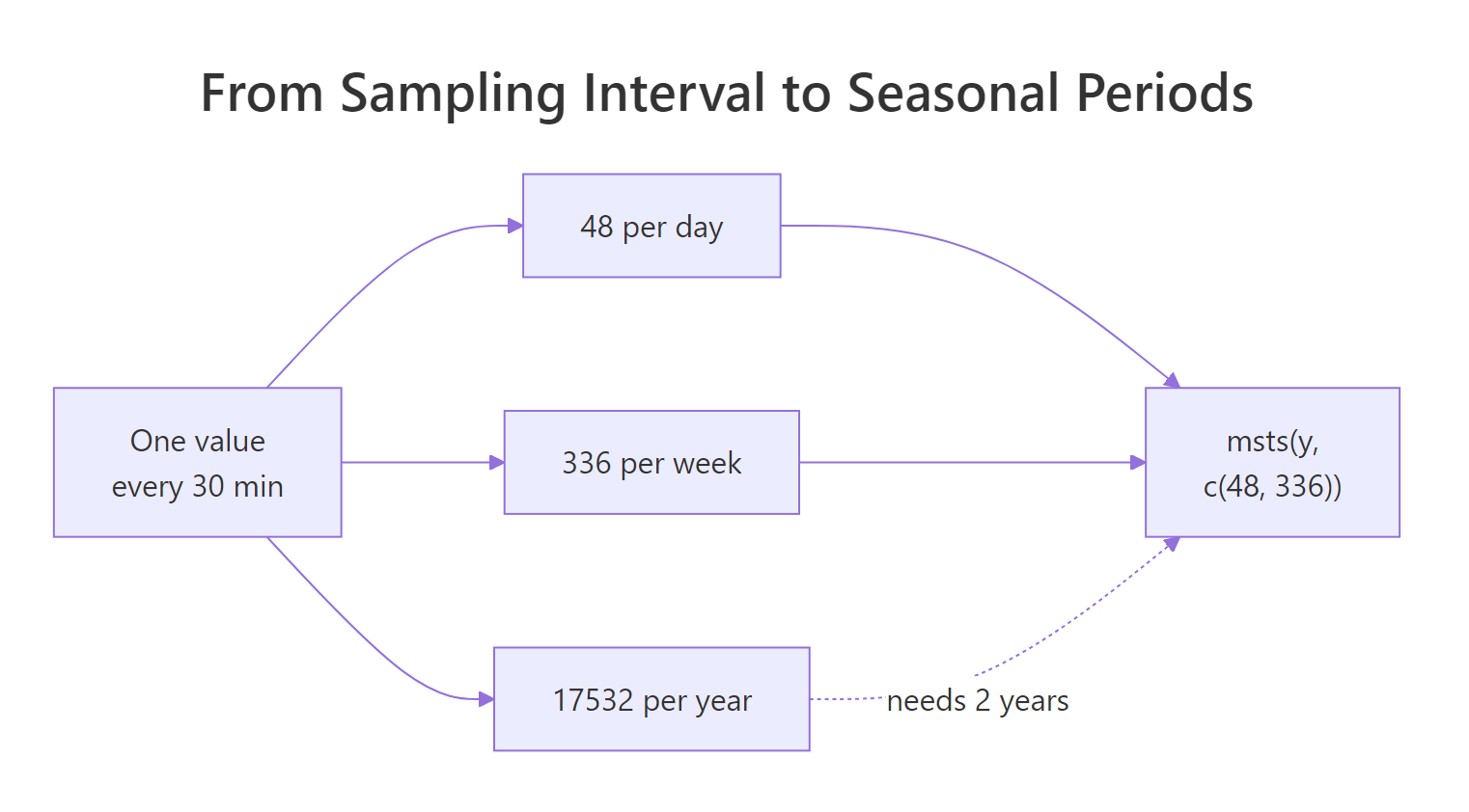
Figure 1: One sampling interval implies several seasonal periods. The annual period exists but needs years of history to estimate.
Arithmetic tells you which periods are possible. It cannot tell you which ones are actually present, and it certainly cannot tell you which ones are strong. For that, look at the autocorrelation function, which measures how similar the series is to a shifted copy of itself. A correlation near 1 at lag k means "the value k steps ago is an excellent guide to the value now".
The acf() call computes correlations at every lag up to 400 and stores them in ac$acf. The + 1 on the index is there because position 1 of that vector holds lag 0, so lag 48 lives at position 49.
Look at the pattern in that last column, because it is the whole argument for multiple seasonality in a single table. Correlation decays as you go back in time: 0.985 half an hour ago, 0.828 yesterday, 0.653 two days ago. Then at 336, a full week back, it jumps back up to 0.910. The same half-hour last week predicts today better than the same half-hour two days ago does. Ordinary decay cannot produce that. Only a genuine weekly cycle can.
One more view is worth having before you model anything, which is the shape of the average day.
Demand sits near 24000 through the small hours, climbs to about 35000 by midday, stays high through the afternoon and evening, and is still at 30330 by ten at night. This is the loud cycle, the one nobody misses.
Try it: Two days back scored 0.653 and one week back scored 0.910. Where does three days back sit? Compute the ACF at lag 144 and compare it with lag 336.
Click to reveal solution
Explanation: Three days back is 0.619, even weaker than two days back at 0.653. The correlation keeps decaying right up until the weekly cycle brings it back. This is the signature of multiple seasonality: a series of decaying values interrupted by a sharp revival at the longer period.
How do you tell R about more than one seasonal period?
You have two containers to choose from, depending on which forecasting ecosystem you are in. The forecast package uses msts(), which is a ts that carries a vector of periods instead of a single number. The tidier fable ecosystem uses a tsibble, which carries real timestamps and works out the periods from them.
We already built the msts version above. Here is what it is holding.
The first line shows both periods stored side by side, exactly as we asked. The second line is the trap. frequency() is the old single-period accessor, and when there are several periods it returns only the largest one. If you check your data with frequency() and see 336, that does not confirm the daily cycle is being modelled. Always check attributes(x)$msts instead.
Printing the object shows the periods in the header, which makes it easy to sanity-check in passing.
The alternative container attaches genuine timestamps to each reading. That costs a little more setup and buys you real calendar awareness, which matters a great deal once holidays and clock changes enter the picture.
Notice the [30m] in the header. The tsibble worked out the sampling interval by itself, from the timestamps, which means it can also tell you whether any readings are missing.
We write tsibble::interval() explicitly because lubridate also exports a function called interval(), and lubridate was loaded second, so it wins. The gap check returns FALSE, confirming there are no missing half-hours anywhere in the 4032 rows. That is worth knowing before you model, for reasons we will get to in the traps section.
Try it: Build a version of the full series that also records the annual period, then confirm all three periods are stored.
Click to reveal solution
Explanation: R accepts the annual period without complaint, but accepting is not the same as being able to estimate it. With only 4032 observations we hold less than a quarter of one annual cycle, so this third period is decoration. The traps section returns to why that matters.
How does MSTL split the series into its seasonal layers?
Before forecasting, it helps enormously to see the cycles separated out. MSTL does exactly that. It runs the classic STL decomposition once per seasonal period, peeling off one layer at a time, shortest period first, and leaves you with a trend, one seasonal column per period, and whatever is left over.
One column per period, named after the period itself, which makes the output self-documenting. Seasonal48 is the daily shape and Seasonal336 is the weekly shape.
The really useful question is how much of the movement each layer explains. Comparing each column's variance with the variance of the original series answers it.
The daily cycle accounts for 73.8 percent of the variance, the weekly cycle for 23.2 percent, the trend for barely 1 percent, and the leftover noise for 0.3 percent. This series is almost entirely seasonal.
That 23.2 percent is the answer to the puzzle from the first section. A model that knows only the daily period is throwing away nearly a quarter of the explainable movement, which is precisely why its forecast error was eleven times worse.
The layers are additive, so they sum back to the original.
Take the first row. The trend sits at 30213.7. It is just after midnight, so the daily component pulls demand down by 5816.4. It is a Monday early morning, so the weekly component pulls it down another 1765.3. The remainder trims 370. Add those four numbers together and you get 22262, which is the observed value in the Data column.
Decomposition is not just diagnostics. It also gives you a forecasting method directly, via stlf(): forecast the seasonally adjusted series with exponential smoothing, then add the seasonal shapes back on.
A MAPE of 2.44 percent, on the same weekend holdout that broke the daily-only model. It is a genuinely good forecast, and worth noting that it is still not as good as the 1.74 we got from the plain seasonal naive. Hold that thought, because the bake-off section takes it seriously.
Try it: Run mstl() on daily_only, the version that only knows about the 48-step period, and look at which columns come back.
Click to reveal solution
Explanation: There is no Seasonal336 column. The weekly variation has not vanished, it has been swept into Trend and Remainder, where no forecasting method can use it as a repeating pattern. That is the mechanism behind the 19 percent error.
How does dynamic harmonic regression fit several cycles at once?
Decomposition handles seasonality by subtracting it. The other main strategy is to describe it, using smooth waves, and then run an ordinary regression. This approach is called dynamic harmonic regression, and it is the workhorse for sub-daily data because it scales to long periods that would choke a seasonal ARIMA.
The idea is simpler than the name suggests. Any repeating shape, however lumpy, can be built by stacking sine and cosine waves of the right sizes. The first pair completes exactly one cycle per period, the second pair completes two cycles per period, the third completes three, and so on. Add enough pairs and you can trace any shape you like. The number of pairs you use is called K, and it is the one knob you turn.
fourier() builds these columns for you, one set per seasonal period.
K = c(2, 1) asks for two pairs for the daily period and one pair for the weekly period, which gives six columns in total: S for sine, C for cosine, the number for which harmonic, and the suffix for which period. The rows match the training data.
These are just numbers, so you can look at them.
S1-48 climbs slowly, 0.131 then 0.259 then 0.383, because it is completing one full wave over 48 steps. S2-48 climbs twice as fast because it completes two waves over the same 48 steps. Regression then picks a coefficient for each column, and the weighted sum of all the waves becomes the fitted seasonal shape.
Now fit one. tslm() is a time-series-aware linear model, so we can regress the series directly on the Fourier columns.
To forecast, we generate the same Fourier columns for the future using the h argument, then hand them over as newdata. Because sine and cosine waves are entirely deterministic, we always know their future values exactly, which is the reason this method extends so comfortably to long horizons.
But 6.09 percent is poor, worse than the plain seasonal naive by a factor of three. The problem is K = 5 for the weekly period. Five wave pairs across a week produce a very smooth shape, smooth enough to say "weekends are lower on average" but nowhere near flexible enough to give weekends a different daily profile. Give the weekly period far more harmonics and it gains that freedom.
The error drops from 6.09 to 2.52 percent, purely from letting the weekly shape be more detailed. Nothing else changed.
You should not pick K by trying values against the test set, though, because that quietly turns your holdout into training data. The honest way is a criterion computed on the training data alone. CV() reports several, and AICc is the one to use here: it rewards fit and penalises extra columns, so it will stop you before you add waves that only chase noise.
Lower is better, so AICc prefers the larger K by a wide margin, agreeing with the holdout without ever having seen it. That agreement is what gives you confidence the choice will hold on future data.
Try it: Try an in-between setting, K = c(8, 25), and compare its AICc against the two above.
Click to reveal solution
Explanation: At 53009.4 this sits between the two, better than c(10, 5) and worse than c(15, 40). AICc is behaving smoothly, which is what makes a grid search over K worthwhile.
Why the prediction intervals are wrong without ARMA errors
The harmonic model gives respectable point forecasts. Its uncertainty estimates, however, are badly broken, and the reason is worth understanding because it applies to every regression you fit on a time series.
Ordinary regression assumes the errors are independent, meaning that knowing today's error tells you nothing about tomorrow's. On half-hourly demand data that assumption is not slightly wrong, it is spectacularly wrong.
The correlation between consecutive residuals is 0.953. If the model is running 500 megawatts too low right now, it will almost certainly still be running too low half an hour from now. The errors arrive in long runs, not as independent scatter.
The fix is to model the leftover structure instead of treating it as noise. Keep the same Fourier columns as regressors, but let the error term follow an ARIMA process instead of assuming it is white noise. White noise means errors drawn independently at every step, with no memory of what came before. An ARIMA error process is the opposite: today's error is built partly from the errors immediately preceding it, which is exactly the behaviour the 0.953 above is reporting.
We pass the Fourier columns through xreg, which is where Arima() expects external regressors, and specify order = c(2, 0, 0). Those three numbers are the count of AR terms, the number of differences, and the count of MA terms, so this asks for an AR(2) error process and nothing else: each error is predicted from the two errors immediately before it. Residual correlation collapses from 0.953 to 0.014, which is effectively zero. The model now accounts for the runs.
Note that this block takes appreciably longer to run than the earlier ones, perhaps twenty seconds or so, because estimating an ARIMA with several dozen regressors over 3936 observations is real work. That cost is a recurring theme with this method.
Now look at what changed in the intervals.
The plain regression gives a 95 percent interval 3348 megawatts wide for the very next half-hour, and exactly the same 3348 for two days out. That is nonsense on its face. Forecasting thirty minutes ahead is obviously easier than forecasting two days ahead, and any honest interval has to widen as the horizon grows.
The ARMA version behaves properly. It starts narrow at 1033, because the AR(2) term predicts the next error from the two most recent residuals, which have already been observed, then widens to 3323 by step 96 as the influence of those residuals decays away. Same point forecasts, sane uncertainty.
And what did all this buy in point accuracy? Almost nothing.
3.13 percent, slightly worse than the 2.52 from the simpler c(15, 40) fit, mostly because we used fewer weekly harmonics here to keep the runtime tolerable. The lesson is that ARMA errors are a fix for your uncertainty estimates, not a route to better point forecasts. If all you publish is a single number, you may not need them. If anyone downstream makes decisions from your intervals, you do.
Try it: The comparison above used 95 percent intervals, which live in column 2 of upper and lower. Column 1 holds the 80 percent intervals. Report the width of the 80 percent interval for the first forecast step.
Click to reveal solution
Explanation: 675 megawatts against 1033 for the 95 percent interval. A narrower interval is a weaker claim: you are saying the truth lands inside it four times in five rather than nineteen times in twenty.
When is TBATS worth the extra runtime?
TBATS is the fully automatic option, and its selling point is that it decides almost everything for you. The name packs in what it can use: Trigonometric seasonality, Box-Cox transformation, ARMA errors, Trend and Seasonal components. Crucially, it lets the seasonal shape drift slowly over time rather than forcing it to stay fixed, which is something neither MSTL nor harmonic regression does by default.
The catch is speed. By default tbats() searches many combinations, with and without the Box-Cox transformation, with and without a trend, with and without ARMA errors, and fits each one. On a long sub-daily series that adds up fast. Restricting the search to a single configuration keeps it manageable.
Each use.* argument switched off removes a branch from the search. This restricted fit takes roughly ten seconds and lands at 4.36 percent.
For comparison, the unrestricted tbats(both) on this same training data took 172 seconds on a normal laptop and scored a MAPE of 7.38, which is worse. The extra search space cost nearly three minutes and bought a less accurate forecast on this particular series. That will not always be the outcome, but it is a useful reminder that "automatic" is not a synonym for "better".
Try it: All these MAPE values need a scale. Fit the worst reasonable benchmark, meanf(), which predicts the historical mean forever, and see what a completely seasonality-blind forecast scores.
Click to reveal solution
Explanation: 16.73 percent for a forecast that uses no seasonality at all. The period-48 seasonal naive scored 19.02, which is worse than the flat mean. Using the wrong seasonal period was more damaging than using none, because it confidently repeated weekday shapes onto a weekend.
Which model actually wins on your data?
Six candidates are now fitted on identical training data and scored against the identical holdout. Putting them in one table is the only way to answer the question honestly.
MASE is worth reading alongside MAPE. It compares your forecast against a naive one-step benchmark, so a MASE below 1 beats that benchmark and above 1 loses to it.
The ordering is uncomfortable and completely real. The plain seasonal naive with the correct period wins outright, and the models get worse as they get more sophisticated. The most expensive model in the table is the least accurate one that knows about weeks.
Before generalising from that, check whether the ranking is an accident of the two-day horizon. Refit on a shorter training set and forecast a full week.
Same ordering over a full week, so it was not a fluke of the weekend window.
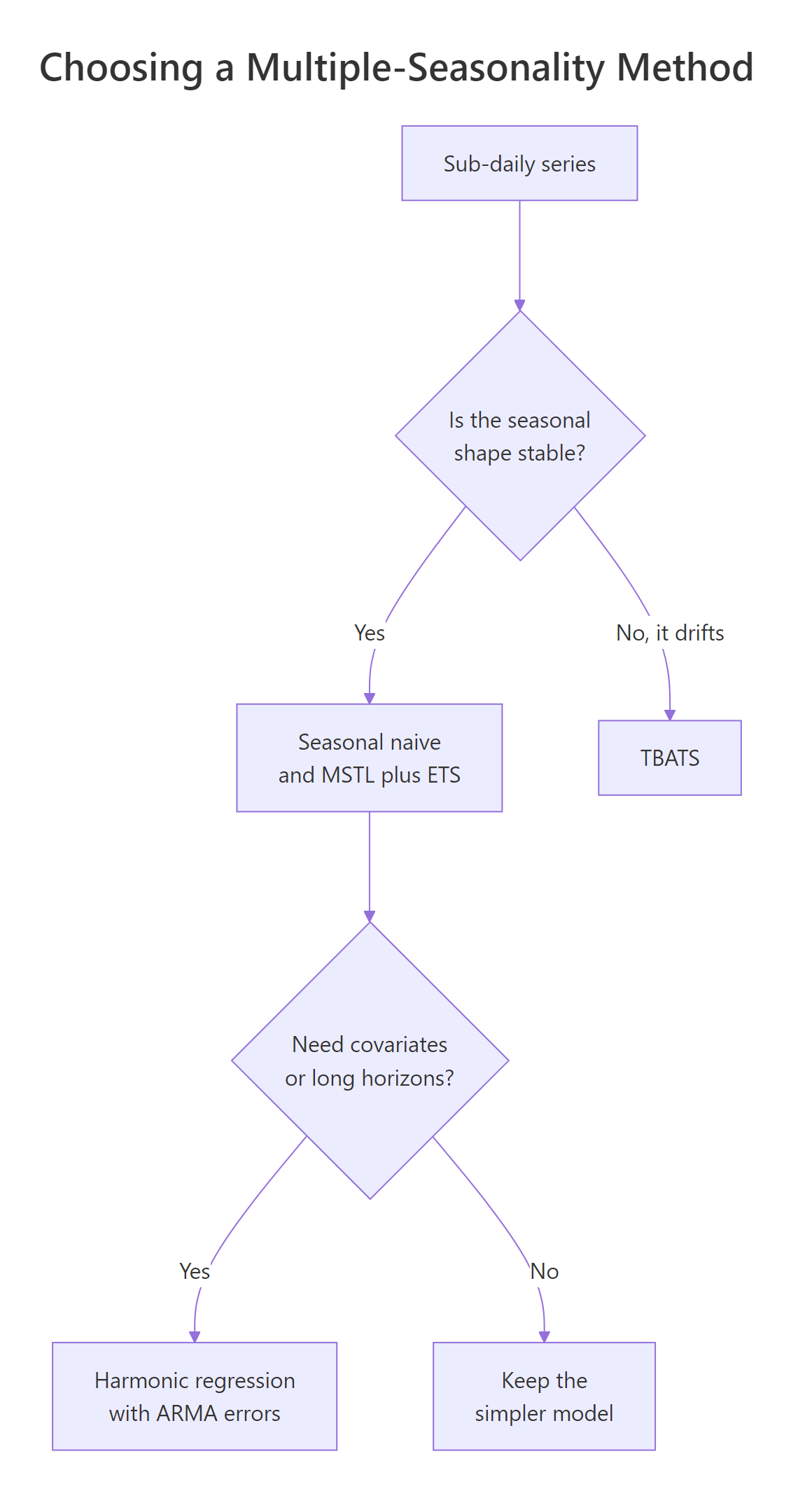
Figure 2: Which multiple-seasonality method to reach for, and what decides it.
Now, this result deserves an honest caveat rather than a victory lap. The taylor series is twelve consecutive summer weeks with no public holidays, no clock change and no year-on-year drift. It is about as friendly as a real series gets, and friendly series are exactly where simple methods shine. Here is where the more elaborate options do earn their keep.
| Method | Reach for it when |
|---|---|
| Seasonal naive (longest period) | Always, as the benchmark. Sometimes it just wins. |
MSTL and stlf() |
You want to see the layers, and the seasonal shape is stable. |
| Harmonic regression | You need covariates (temperature, holidays, promotions), long horizons, or many seasonal periods at once. |
| Harmonic plus ARMA errors | Anyone downstream uses your prediction intervals. |
| TBATS | The seasonal shape drifts across months or years, and you can afford the runtime. |
The one thing every row shares is that you cannot know which applies to your series without doing what we just did.
Try it: The one-week check above scored only two methods. Add the harmonic regression to it and find out whether the ranking survives the longer horizon as well.
Click to reveal solution
Explanation: 0.81 MASE, still third behind the seasonal naive at 0.57 and MSTL at 0.69, so the ordering is the same over a week as it was over a weekend. Notice also that the harmonic model improves in absolute terms at the longer horizon, from 2.52 percent to 1.79, because the week-long window contains five ordinary weekdays it predicts easily rather than two awkward weekend days.
What sub-daily traps will break your model?
Sub-daily data has failure modes that monthly data simply does not have, and every one of them is quiet. Nothing errors. You just get a worse forecast than you should and no clue why.
Trap one: the clocks change. Every msts model assumes a fixed number of observations per cycle. Daylight saving time breaks that assumption twice a year.
In March the clocks go forward and the day holds 46 half-hours. In October they go back and it holds 50. If you store local time and assume 48 per day, then from the last Sunday in March onwards every observation sits in the wrong seasonal slot, permanently. The standard defence is to store and model in UTC, where every day really does have 48 half-hours, and handle the local-time effect as a separate regressor if the behaviour genuinely follows the wall clock.
Trap two: missing rows shift everything after them. Because the seasonal period is a count of rows, one dropped reading moves every later observation one slot out of alignment.
Ten readings removed and the tsibble reports it immediately. A plain vector carries no timestamps, so neither it nor msts() has any way to detect the loss. The repair is to restore the full time grid, which converts a silent misalignment into visible missing values.
Back to 4032 rows with 10 explicit NAs. Now every reading is in its correct seasonal slot again, and you can decide how to impute the gaps as a separate, deliberate step.
has_gaps() before you build the series.Trap three: you cannot estimate a cycle you have not observed twice. The annual period is real for electricity demand, but reality is not enough.
84 daily cycles and 12 weekly cycles are plenty. 0.23 of an annual cycle is not a cycle at all, it is a fragment. Include the annual period anyway and the model will happily fit summer's upward slope and then extrapolate it into a fictional winter. As a rule of thumb, you want at least two complete cycles before a period is worth modelling, and preferably more.
Trap four: nested periods overlap. A week contains exactly seven days, so harmonic 7 of the weekly period is mathematically identical to harmonic 1 of the daily period. Include both and the regression is singular.
We asked for 8 weekly harmonics and got 7 back. Read the sequence carefully: it runs 1 through 6, then skips straight to 8. S7-336 and C7-336 are absent because they duplicate S1-48 and C1-48, and fourier() drops them automatically without printing a message. This is helpful behaviour, but it means your model has slightly fewer columns than you asked for, so do not be surprised when the count does not match your arithmetic. Some other packages warn about the same collision instead of silently dropping it.
Try it: Practise the gap-repair workflow on a different slice. Remove readings 500 to 520 from elec, restore the grid, and count the resulting missing values.
Click to reveal solution
Explanation: 21 rows removed gives 21 NAs after repair. The count always matches, which makes this a quick integrity check: if fill_gaps() adds more rows than you expected, your timestamps have a problem beyond simple missing readings.
Complete Example: the five-step playbook end to end
Here is the whole method on one series, start to finish. Step one is arithmetic: derive the candidate periods from the sampling rate, and check you hold enough cycles of each to bother.
84 daily cycles and 12 weekly cycles, both comfortably above the two-cycle minimum. The annual period is dropped here rather than carried along as decoration.
Step two and three: hold out the final two days and score a shortlist on them. The shortlist deliberately starts with the benchmark.
Sorting by MASE puts the winner on top automatically, so the choice is made by the numbers rather than by preference.
Step four and five: refit the winner on every observation you have, including the holdout, and produce the forecast you actually ship.
The next 24 hours of demand with 95 percent intervals, from a model chosen on evidence rather than fashion. Refitting on the full data before shipping matters: the holdout existed to choose the model, and once that choice is made you want the final model to have seen every observation available.
Practice Exercises
Exercise 1: Does the weekend explain the whole gap?
The period-48 model scored 19.02 percent against a Saturday and Sunday holdout. Test whether that failure is specifically about weekends. Move the holdout back two days so it covers Thursday and Friday instead, then compare the period-48 and period-336 models on that midweek window. The series has 4032 observations and starts on a Monday.
Click to reveal solution
Explanation: 1.25 against 1.11. The daily-only model nearly catches up, because midweek days genuinely do resemble each other, so repeating Wednesday onto Thursday works fine. The weekly period only pays off when the forecast window crosses a boundary between day types. This is why a holdout that never spans a weekend would have hidden the problem completely, and why you should always check that your evaluation window contains the situations you actually care about.
Exercise 2: Pick K properly with a grid search
Choosing K by trying values against the test set is cheating. Do it the honest way instead: scan a grid of K settings, compute AICc for each on the training data alone, and report the table. Use both as the series and try c(10,10), c(10,20), c(15,30), c(15,40) and c(20,50).
One warning that will save you a confusing error. tslm() looks up the variables in your formula by name, so if you call it with the K value hidden inside an anonymous function (sapply(grid, function(k) tslm(both ~ fourier(both, K = k)))) it will fail with "object 'k' not found". Use a plain for loop so the variable lives where tslm() can find it.
Click to reveal solution
Explanation: AICc falls to a minimum of 52723.2 at c(15, 40) and then rises again at c(20, 50). That turning point is the important part. More harmonics are not automatically better, and the criterion found the balance without ever touching the holdout. This is also the setting that scored best on the test set earlier, which is exactly the agreement you hope to see.
Exercise 3: Diagnose an unfamiliar series
Someone hands you eight weeks of hourly readings and tells you nothing about them. Recover the seasonal structure yourself. Build the series below, then use the ACF to confirm which periods are present, and decompose it to check your answer.
Click to reveal solution
Explanation: Strong correlation at both lag 24 and lag 168 confirms a daily and a weekly cycle, which matches how the series was built. Note that the periods are 24 and 168, not 48 and 336, because these are hourly readings rather than half-hourly. The period always depends on the sampling rate, never on the calendar alone. Decomposing with both periods recovers a Seasonal24 and a Seasonal168 column, closing the loop on the diagnosis.
Frequently Asked Questions
Do I have to use msts, or will a plain ts work? A plain ts holds exactly one seasonal period, so it works only if your data genuinely has one. For sub-daily data that is almost never true. Use msts() for the forecast package or a tsibble for fable.
I built a tsibble. How do I actually forecast it? Every model in this tutorial comes from the forecast package and wants an msts object, so the tsibble here was used for its calendar checks (interval(), has_gaps(), fill_gaps()) rather than for fitting. To model the tsibble directly you use the fable package instead, where the same three ideas appear as STL(), TSLM(demand ~ fourier(period = 48, K = 15) + fourier(period = 336, K = 40)) and ARIMA() with Fourier regressors. A common and perfectly reasonable workflow is to clean and check the series as a tsibble, then hand the demand column to msts() for fitting.
How many seasonal periods is too many? Include a period only if you hold at least two complete cycles of it and the ACF shows a bump at that lag. In practice sub-daily series use two, the day and the week. The annual cycle needs several years of history before it is worth the parameters.
What about prophet? Prophet handles multiple seasonalities via Fourier terms too, and is available in R through the fable.prophet package. It is convenient with holidays and missing data, but the ideas here are the same ones under its hood, and on regular series it rarely beats a well-specified harmonic regression.
My timestamps are irregular, not on a fixed grid. Everything in this tutorial assumes a fixed interval, because the seasonal period is a count of rows. Aggregate to a regular grid first (round to the nearest five or fifteen minutes), then run has_gaps() and fill_gaps() before modelling.
Should I model the annual cycle if I only have a few months? No. With less than two full annual cycles the model cannot separate the annual shape from the trend, and it will extrapolate whatever slope your sample happens to contain. Wait for the data or capture the effect with covariates such as temperature instead.
Summary

Figure 3: The five steps, in order, for any sub-daily series.
| Step | What you do | The tool |
|---|---|---|
| 1. Count the periods | Multiply observations per hour by the hours in each cycle | Arithmetic |
| 2. Confirm with the ACF | Check for a correlation bump at each candidate lag | acf() |
| 3. Build the container | Store every real period in one object | msts() or tsibble() |
| 4. Score a shortlist | Benchmark first, then MSTL, then harmonic regression | accuracy() on a holdout |
| 5. Refit and forecast | Retrain the winner on all data before shipping | forecast() |
The findings worth carrying away:
- A seasonal period is a count of observations, not a duration. Half-hourly data has 48 per day and 336 per week.
- Getting the period wrong cost more than any modelling choice: 19.02 percent error against 1.74 percent, from the same method on the same data.
- The daily cycle held 73.8 percent of the variance and the weekly cycle 23.2 percent. Discarding the weekly layer discards nearly a quarter of the signal.
- Harmonic regression needs generous K on the longer period, otherwise the weekly shape is too smooth to tell a weekday from a weekend.
- ARMA errors fix prediction intervals, not point forecasts. A flat interval is the symptom.
- TBATS is for seasonality that drifts. On a stable series it costs a lot of runtime for nothing.
- The seasonal naive with the right period beat every sophisticated model here, at both a two-day and a one-week horizon. Fit it first and make everything else prove itself.
References
- Hyndman, R.J. and Athanasopoulos, G. Forecasting: Principles and Practice, 3rd edition. Section 12.1: Complex seasonality. Link
- Hyndman, R.J. and Athanasopoulos, G. Forecasting: Principles and Practice, 2nd edition. Section 11.1: Complex seasonality, covering
msts,mstlandtbats. Link - De Livera, A.M., Hyndman, R.J. and Snyder, R.D. Forecasting time series with complex seasonal patterns using exponential smoothing. Journal of the American Statistical Association 106(496), 1513-1527 (2011). The original TBATS paper. Link
- Hyndman, R.J. Seasonal periods. Hyndsight blog, on choosing periods for weekly, daily and sub-daily data. Link
- forecast package reference:
msts(), multi-seasonal time series objects. Link - forecast package reference:
tbats(), and itsuse.*search arguments. Link - tsibble documentation:
fill_gaps(), and how implicit missing values differ from explicit NA. Link - Hyndman, R.J. and Athanasopoulos, G. Forecasting: Principles and Practice, 3rd edition. Section 10.5: Dynamic harmonic regression. Link
Continue Learning
- Fourier Terms in R goes much deeper on harmonic regression: what each sine and cosine pair contributes, how to select K, and how to fit the same models in fable.
- MSTL in R covers multiple seasonal decomposition on its own terms, including how to read and adjust the seasonal windows.
- Backtesting Forecasts in R replaces the single holdout used here with rolling-origin evaluation, which is the more reliable way to choose between close candidates.