auto.arima() in R: How It Works and When to Override It
auto.arima() automates the whole ARIMA-building recipe: it runs statistical tests to decide how much to difference the data, then searches many model orders and returns the one with the lowest AICc, already fitted by maximum likelihood. It is an excellent default, but it optimises a formula rather than your forecast, so knowing when to override it is the skill that matters.
What does auto.arima() actually do when you call it?
Suppose you have a series and you want a forecast today, not a week of ACF-plot study. That is exactly what auto.arima() is for. One call reads the data, decides the differencing, tries a family of ARIMA models, and hands back the best one it found, already estimated. Let us call it on real data and see what comes back.
We will use WWWusage, a built-in series of 100 minute-by-minute counts of users connected to a server. It comes with the forecast package, so loading the package makes it available.
The one line auto.arima(WWWusage) did three separate jobs. It decided the series needed one difference (the 1 in the middle of ARIMA(1,1,1)), it picked one autoregressive term and one moving-average term (the outer numbers), and it estimated the coefficients you see under Coefficients. The ARIMA(1,1,1) label is the model it chose; everything else is the fit.
Behind that single call is a fixed sequence of steps. It always runs them in the same order, and the rest of this tutorial walks through each one so you can see where its judgment can go wrong.

Figure 1: The five internal steps auto.arima() runs on every call.
A fitted model is only useful if you can forecast from it. The forecast() function takes the model and a horizon h and returns point forecasts plus prediction intervals.
Each row is one step into the future. The Point Forecast column is the model's best single guess, and the four columns beside it give the 80% and 95% prediction intervals. Notice how the intervals widen the further out you go: forecast 101 spans about 12 units at the 95% level, while forecast 110 spans about 140. The intervals widen because the model is genuinely less sure about ten steps ahead than about one, and that is the behaviour you want to see.
You can see the same thing as a picture with a fan chart, which draws the point forecast as a line and the intervals as shaded bands.
The chart shows the historical series rising and levelling off, then the forecast continuing that level with a grey fan that flares out over the ten-step horizon. Seeing the fan makes the growing uncertainty obvious at a glance.
Try it: Call auto.arima() on the built-in lh series (48 readings of a luteinising hormone level). What order does it choose, and did it difference the data at all?
Click to reveal solution
Explanation: The middle number is 0, so auto.arima() did not difference lh at all. It chose ARIMA(1,0,0), a single autoregressive term plus a mean, because the series is already stationary and hovers around a fixed level.
What does auto.arima() try to minimise (AIC, AICc, or BIC)?
When auto.arima() says one model is better than another, it means one specific thing: the better model has a lower information criterion. By default that criterion is the AICc, and understanding it explains almost every choice the function makes.
An information criterion scores a model on two things at once. It rewards a model for fitting the data well, and it punishes the model for every extra coefficient it uses. A model that fits slightly better but needs three more terms to do it will usually lose. The score is a single number, and lower is better.
You can read the score straight off any fitted model.
The print-out of the model showed three related numbers on its last line, and you can pull all three at once. AIC is the base score, AICc is the same idea with a small-sample correction, and BIC punishes complexity more harshly.
For this model the three scores are close, which is common. The gaps only matter when you compare competing models: a difference of less than about 2 in AICc means the two models have similar support from the data, so you should not agonise over which to pick.
If you have a reason to prefer a different criterion, the ic argument switches it. BIC, for example, leans harder against extra terms and tends to pick smaller models on long series.
Here BIC lands on the same ARIMA(1,1,1) as the default, because the series is short and the two criteria agree. On a longer series they can diverge, with BIC preferring the more parsimonious model.
If you like the underlying maths, the AICc adds a correction term to the ordinary AIC. You can skip this box; the code above is all you need to use the function well.
$$\text{AICc} = \text{AIC} + \frac{2k(k+1)}{n - k - 1}, \qquad \text{AIC} = -2\ln(L) + 2k$$
Where:
- $L$ is the maximised likelihood of the model, a measure of how well it fits
- $k$ is the number of estimated parameters
- $n$ is the number of observations
The extra fraction is the correction. When $n$ is large it shrinks toward zero and AICc behaves like AIC, but when $n$ is small it grows and penalises extra parameters more sharply.
Try it: Read all three information criteria off your WWWusage model in one line, rounded to two decimals.
Click to reveal solution
Explanation: Each criterion lives inside the fitted model object under its own name, so combining them into a named vector prints a tidy one-line summary. AICc sits just above AIC, and BIC is highest because it charges the most for the two coefficients.
How does auto.arima() decide how much to difference?
Differencing is how ARIMA removes a trend: instead of modelling the raw levels, it models the change from one step to the next. The number of times it differences is the d in the middle of the order, and auto.arima() does not search for d the way it searches for the other terms. It decides d first with a statistical test, and only then searches the rest.
The test is the KPSS test, which asks whether a series is stationary (has a stable mean over time). auto.arima() runs it, and if the series fails, it differences once and tests again, repeating until the series passes or it hits the limit of two differences. The helper ndiffs() runs exactly that procedure and reports the answer.
The answer is 1, which is why every WWWusage model above had a 1 in the middle. The series drifts upward, so one difference is needed to flatten it into something stationary.
Seasonal data needs a second kind of differencing. A monthly series with a yearly pattern often needs to be compared against the same month last year, which is a seasonal difference, written as the capital D. auto.arima() picks D with its own seasonal-strength test, and nsdiffs() reports it. Let us check both counts for AirPassengers, the classic monthly airline series with strong yearly seasonality.
Both come back as 1, so auto.arima() will apply one ordinary difference and one seasonal difference to AirPassengers before it searches for the seasonal and non-seasonal AR and MA terms. That matches what a person would do by eye: remove the upward trend, then remove the repeating yearly shape.
Try it: How much differencing does auto.arima() apply to austres, a quarterly count of Australian residents? Report both the ordinary count d and the seasonal count D.
Click to reveal solution
Explanation: austres climbs steadily and its trend itself changes slope, so one difference is not enough to flatten it and the KPSS procedure asks for a second, giving d = 2. There is no repeating quarterly shape once the trend is gone, so the seasonal count is 0.
How does the stepwise search find a model, and when does it get stuck?
Once d and D are fixed, auto.arima() has to choose the AR and MA orders, and here is where its speed comes from. Rather than fit every possible combination, it uses the stepwise search from the Hyndman-Khandakar algorithm, which behaves like climbing a hill in fog: it starts at a few points, then keeps stepping toward whatever is better nearby.
The search begins by fitting four starting models, ARIMA(0,d,0), ARIMA(2,d,2), ARIMA(1,d,0), and ARIMA(0,d,1), and keeping the best. From there it only ever looks at close neighbours of the current best: it nudges p or q up or down by one, or flips the constant term on or off, and moves to any neighbour that lowers the AICc. When no neighbour improves, it stops.
You can watch the whole climb by passing trace = TRUE, which prints every model it tries with its AICc.
Read the trace from the top. It began near ARIMA(2,1,2), wandered through neighbours, and settled on ARIMA(1,1,1) at an AICc of 514.55 because nothing one step away scored lower. That is the model it returned at the very start of this tutorial. The search tried 18 models out of the dozens that were possible.
Now watch what happens when you force it to try every model instead of walking the hill. Setting stepwise = FALSE searches the full grid, and approximation = FALSE uses the exact likelihood rather than a fast approximation.
The exhaustive search found ARIMA(3,1,0), a different model, and its AICc is lower. Line the two scores up to see the gap.
The full search beats the stepwise search by about 2 points of AICc. Look back at the trace: ARIMA(3,1,0) never appears in it. The stepwise walk started around p = 2 and drifted toward smaller models, so it never stepped out to three autoregressive terms with zero MA terms. The better model was sitting in a direction the hill climb never looked.
The approximation shortcut is the second speed trick. To score models quickly during the search, auto.arima() can use an approximate likelihood, then re-estimate only the winner exactly. That is a sensible default for long or highly seasonal series where exact fitting is slow, but it means the score used to compare models is itself approximate, which can tip a close race the wrong way.
Try it: Run the exhaustive search on lh with stepwise = FALSE and approximation = FALSE. Does it pick a different order than the default ARIMA(1,0,0) you found earlier?
Click to reveal solution
Explanation: The full search prefers ARIMA(0,0,2), two moving-average terms, over the default's single autoregressive term. Its AICc of 63.99 beats the default's 65.30, so once again the exhaustive search squeezed out a slightly better model that the stepwise walk missed.
When should you override auto.arima()?
auto.arima() is a strong starting point, not a final answer. There are four recurring situations where its default choice is worth overriding, and each has a specific fix. The figure below maps them out, and the rest of this section works through them one at a time.
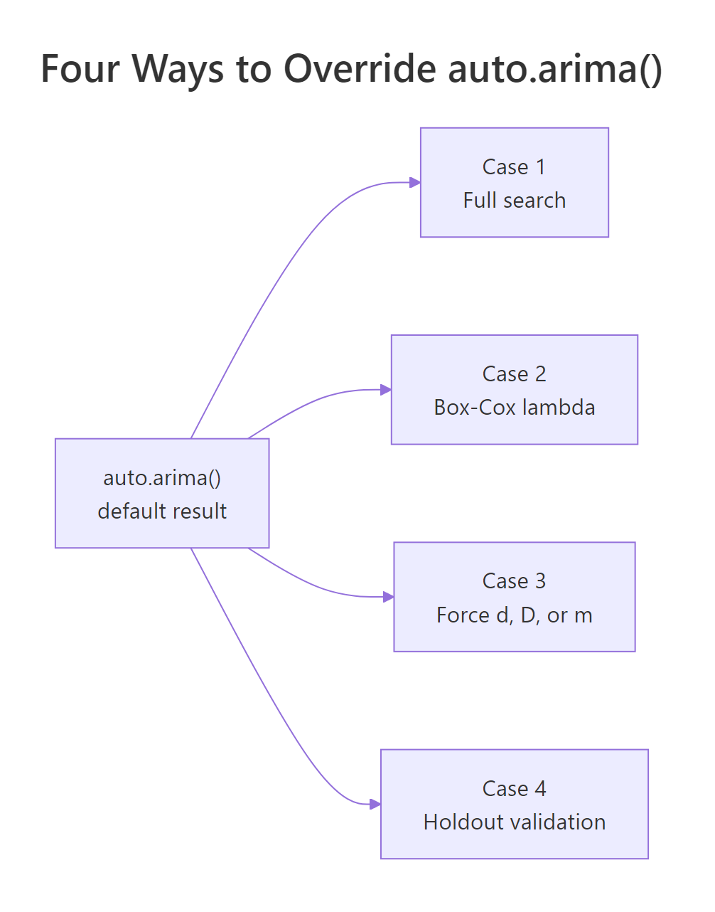
Figure 2: The four situations where you should override the default.
Case 1: You are analysing a single important series
You already saw this one. The default stepwise search trades accuracy for speed so it can process thousands of series in a batch. When you care about one series, spend the extra seconds on the full search, exactly as you did for WWWusage, where the exhaustive search found ARIMA(3,1,0) at an AICc of 512.42 against the stepwise ARIMA(1,1,1) at 514.55. The fix is stepwise = FALSE, approximation = FALSE, and it should be your default habit for any model that matters.
Case 2: The variance grows as the level grows
Look at what auto.arima() picks for AirPassengers with no help.
The AirPassengers series has a well-known quirk: the size of its yearly swings grows as the numbers grow, so the wobble in 1960 is much bigger than in 1949. ARIMA assumes the wobble stays a constant size, so fitting the raw series breaks that assumption. A Box-Cox transformation fixes this by squashing large values more than small ones, which evens out the variance. Setting lambda = "auto" lets auto.arima() choose the transformation strength for you.
With the variance evened out, auto.arima() lands on ARIMA(0,1,1)(0,1,1)[12], the famous "airline model" that textbooks fit to this exact series by hand. The transform changed the answer because it changed the shape of the data the search was looking at. When your series fans out as it climbs, a transform is usually the right move.
Case 3: You know a structure the search got wrong
Sometimes you know something about the data that the automatic tests do not. auto.arima() lets you pin down any part of the model and search the rest. You can force the differencing with d and D, switch seasonality off with seasonal = FALSE, or cap the orders with arguments like max.p.
These overrides are powerful, and that means they can also hurt. Turn off seasonality on AirPassengers, a deeply seasonal series, and watch the fit fall apart.
Without seasonal terms, the model uses four autoregressive terms to approximate the yearly pattern and still scores an AICc of 1357, far worse than the 1018 of the seasonal fit. The lesson is not "never override"; it is "override when you have a reason." A good reason to force d, for instance, is a series where you know a difference is needed for economic reasons even if the test disagrees. A bad reason is a guess. Here is what forcing d = 0 on the trending WWWusage costs you.
Forcing zero differences pushes the AICc up to 526.47 from the differenced model's 514.55, because the model now has to explain the trend with AR terms instead of removing it cleanly. Trust the KPSS test here.
Case 4: The lowest AICc is not the best forecaster
This is the deepest reason to override, and the one people miss. auto.arima() minimises an in-sample score, but your goal is out-of-sample accuracy, and the two are not the same thing. The only way to know which model forecasts better is to hold back recent data and measure the forecast error on it.
Split AirPassengers into a training stretch through 1958 and a test stretch of 1959 onward. Fit the default model and the Box-Cox model on the training data only, then forecast the test period and compare the errors.
The Box-Cox model's forecasts are less than half as wrong: a test-set error (RMSE) of 32 against 74, and an average percentage error of 6.5% against 14.9%. Here is the trap. You cannot see this from the AICc, because the two models were fitted on differently transformed data, so their AICc values are on different scales and simply are not comparable. Only the holdout test reveals which model actually forecasts better.
Try it: Add lambda = "auto" to auto.arima() on USAccDeaths (monthly US accidental deaths) and compare the model order to the default fit. Did the transform change the model this time?
Click to reveal solution
Explanation: Both fits are ARIMA(0,1,1)(0,1,1)[12], so the transform did not change the structure. The chosen lambda is near zero and the variance of this series is already fairly stable, so a transform buys little here. The takeaway is that you cannot assume a transform helps; you test it.
Complete Example: forecasting air passengers end to end
Let us put every idea together and build a real forecast for AirPassengers, the way you would for a model that matters. We will hold out the last two years to test the model honestly, then refit on all the data to forecast the future.
First, fit on the training data with the two overrides that matter for this series: an automatic Box-Cox transform because the variance grows, and the full search because we only have one series to fit.
The training model is the airline model again. Now check how well it forecasts the two held-out years by measuring the error on the test set.
An average error of 6.5% across a two-year forecast is strong for a series with this much growth and seasonality. That is good enough to trust, so the last step is to refit on the full series and forecast the genuine future.
The forecast reproduces the shape of the data: a summer peak around July, a winter dip, and a higher overall level than the year before. Plotting it makes the seasonal fan clear.
That is a complete, defensible workflow. Choose the overrides your data calls for, validate on a holdout, then forecast the future once you trust the model.
Frequently Asked Questions
Does auto.arima() always give the best possible model?
No. It gives the best model its search found under its default shortcuts. The stepwise walk can stop at a local best, and the approximation can misjudge a close race, so a fuller search often finds a slightly better model, as you saw with WWWusage.
Why did auto.arima() pick a different order than my manual ACF and PACF reading?
The two methods optimise different things. Reading ACF and PACF plots identifies plausible orders by eye, while auto.arima() minimises the AICc across many candidates. They often agree, but when they differ, the function is choosing the lower-scoring model, which is not always the one the plots suggest. Our guide to reading ACF and PACF walks through the manual method.
Should I set stepwise = FALSE every time?
Set it whenever you are fitting one series that matters and can spare a few seconds. Keep the default stepwise search when you are fitting many series in a batch, where its speed is the whole point and the small accuracy cost is acceptable.
Can I compare AICc between a model with a Box-Cox transform and one without?
No. A transform changes the scale of the data, so the likelihoods are not measured in the same units and the AICc values are not comparable. Compare those models with out-of-sample accuracy on a holdout instead.
What does "with drift" mean in the output?
Drift is a constant slope added to a differenced model, so the forecast keeps trending instead of levelling off. auto.arima() adds it when a differenced series still has a steady upward or downward march, and it reports "with drift" when it does.
Why did auto.arima() choose a d I did not expect?
Because d comes from the KPSS test, not from the AICc search. If you expected a different amount of differencing, either trust the test or override it directly with the d argument, but remember that forcing the wrong d usually makes the fit worse.
Practice Exercises
These combine several ideas from the tutorial. Try each before opening the solution. The exercises use their own variable names so they will not overwrite the models you fitted above.
Exercise 1: Compare the two searches on a double-differenced series
Fit austres with the default stepwise search and again with the exhaustive search. Report each model's order and its AICc, and note whether the two searches agree. This combines the differencing idea (you already know austres needs d = 2) with the stepwise-versus-full comparison.
Click to reveal solution
Explanation: Both searches land on ARIMA(0,2,1)(1,0,0)[4] with an identical AICc of 652.15. Here the stepwise walk already reached the best model, so the full search only confirms it. That is a useful result: the searches do not always disagree, and when they match you can trust the default with more confidence.
Exercise 2: Test whether a transform actually improves forecasts
Using USAccDeaths, hold out 1978 onward as a test set. Fit the default model and the Box-Cox model on the earlier data, forecast the test period, and compare their test-set RMSE. Decide, from the numbers, whether the transform is worth using here. This combines the Box-Cox override with holdout validation.
Click to reveal solution
Explanation: The default model forecasts slightly better (RMSE 288.83) than the Box-Cox model (294.36). The variance of accidental deaths is fairly stable, so the transform adds nothing and even hurts a little. This is the mirror image of the AirPassengers result, and it is why you validate rather than assume a transform always helps.
Exercise 3: Force a difference the test did not want
Fit lynx, the annual lynx-trapping series, with the default auto.arima(), then force one difference with d = 1. Compare the orders and the AICc of the two fits, and explain why the KPSS test left lynx undifferenced. This combines the differencing decision with a forced override.
Click to reveal solution
Explanation: The default keeps lynx undifferenced at ARIMA(2,0,2) with an AICc of 1876.95, while forcing d = 1 gives ARIMA(0,1,1) and a worse AICc of 1897.45. The lynx series swings up and down in a roughly ten-year cycle but does not trend, so it is already stationary. The KPSS test sees no trend to remove, and forcing a difference throws away information instead of helping.
Summary
auto.arima() automates ARIMA modelling by choosing the differencing with statistical tests, then searching model orders to minimise an information criterion. It is a reliable default, and it becomes far more reliable once you know how to steer it.
| Topic | What to remember |
|---|---|
| What it optimises | The AICc by default; switch with ic. Lower is better; gaps under 2 are ties. |
| How it differences | d from repeated KPSS tests, D from a seasonal test, both fixed before the order search. |
| How it searches | A stepwise hill climb from four start models; fast but can miss a better model. |
| Override 1 | Use stepwise = FALSE, approximation = FALSE for any single important series. |
| Override 2 | Use lambda = "auto" when the variance grows with the level. |
| Override 3 | Force d, D, or seasonality only when you have a real reason; guessing usually hurts. |
| Override 4 | Validate on a holdout, because the lowest AICc is not always the best forecaster. |
The mindmap below gathers the whole picture in one view.
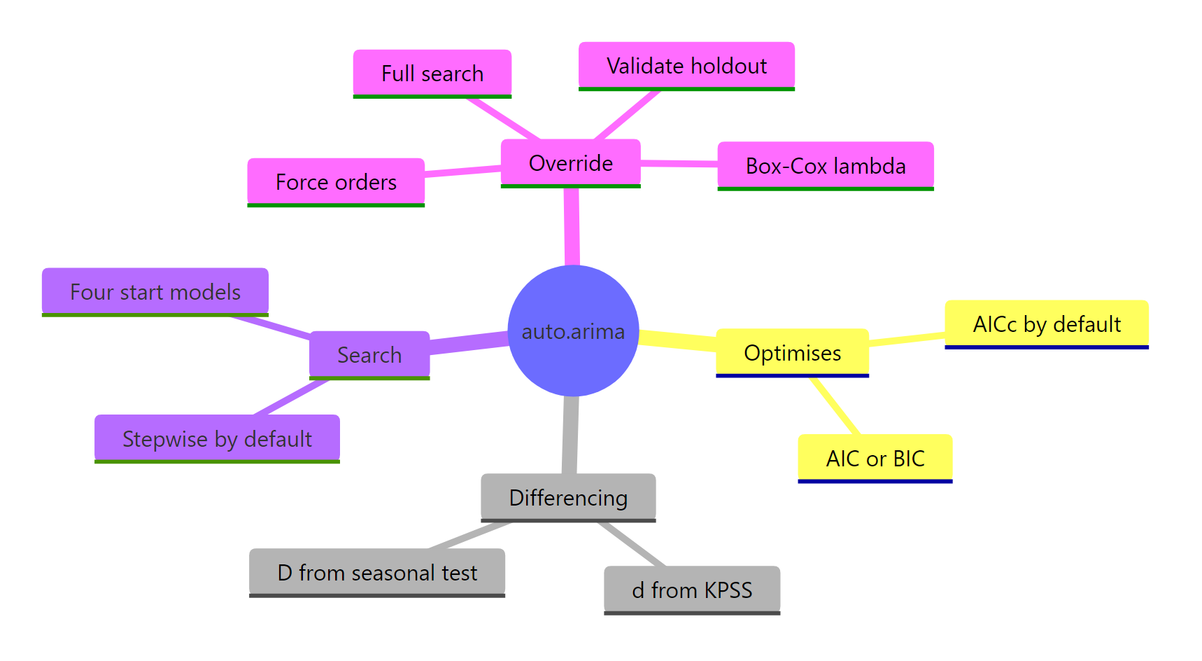
Figure 3: auto.arima() at a glance, from what it optimises to how to override it.
References
- Hyndman, R.J. & Athanasopoulos, G. Forecasting: Principles and Practice (2nd ed), Section 8.7: ARIMA modelling in R. Link
- Hyndman, R.J. & Athanasopoulos, G. Forecasting: Principles and Practice (3rd ed), Section 9.7: ARIMA modelling in R. Link
- forecast package reference: auto.arima(). Link
- Hyndman, R.J. & Khandakar, Y. (2008). Automatic Time Series Forecasting: The forecast Package for R. Journal of Statistical Software, 27(3). Link
- Hyndman, R.J. & Athanasopoulos, G. Forecasting: Principles and Practice (3rd ed), Section 9.1: Stationarity and differencing. Link
- forecast package on CRAN. Link
Continue Learning
- ARIMA in R: What AR, I, and MA Mean and How to Fit One - the foundations behind every order auto.arima() prints, so you can read its output with understanding.
- How to Choose ARIMA Order (p,d,q) in R - the manual ACF and PACF method that auto.arima() automates, worth knowing so you can sanity-check its choices.
- Test Stationarity in R - a closer look at the KPSS and unit-root tests that auto.arima() uses to decide how much to difference.