Time Series Anomaly Detection in R: tsoutliers, anomalize
Time series anomaly detection finds points that break the pattern a series has already established, judging each observation against its own trend and season rather than against the overall mean. In R the tsoutliers package fits an ARIMA model and names each anomaly's shape, telling a one-off spike apart from a permanent level shift, while the anomalize package decomposes a tidy data frame and flags unusual remainders across one series or hundreds at a time.
Why can't a plain z-score find anomalies in a time series?
The Nile has been measured at Aswan every year since 1871, and its most famous feature is a permanent drop in flow around the turn of the century. Ask a z-score to find it and you get nothing at all. That failure is the whole reason time series anomaly detection is a separate subject, so it is worth watching it happen.
A z-score is the standard textbook outlier test. You take each value, subtract the mean of the series, divide by the standard deviation, and flag anything more than three standard deviations away. The Nile dataset ships with R, so you can run this right now.
Read that carefully. sum(abs(nile_z) > 3) counts the years whose z-score is bigger than 3 in either direction, and the answer is zero. The second line asks for the most extreme year in the whole century, and even that one is only 2.74 standard deviations out. By the textbook rule, this series is completely clean.
It is not clean. Plot it and the problem is obvious.
Figure 1: The Nile series drops to a visibly lower level after 1899 and never recovers. Construction of the Aswan Low Dam began in 1898.
The series does not have a spike. It has a step. Everything after the dashed line lives at a lower level than everything before it, permanently. Let us put a number on it.
window() cuts a slice out of a time series by date, so the first line averages every year up to 1898 and the second averages every year from 1899 on. The gap is 248 units, which is about one and a half standard deviations of the whole series.
Here is why the z-score missed it. The mean it subtracts, roughly 1,098 before the break and 850 after, is a single blended number computed from both halves at once. Every individual year sits close to that blend, because the shift is smaller than the year-to-year noise. No single point is extreme. The pattern is extreme, and a z-score cannot see patterns.
Trend is one way a series hides its anomalies. Season is the other, and for that we need data with a repeating cycle. The anomalize package ships with 425 days of real CRAN download counts for 15 tidyverse packages, which is exactly that kind of data.
Two pieces of that block may be new to you. suppressPackageStartupMessages() hides the banner a package prints while it loads, so the output above stays readable; delete it and nothing else changes. |> is R's native pipe: x |> f() is another way of writing f(x), and chaining it lets you read a sequence of steps top to bottom instead of inside out.
tidyverse_cran_downloads arrives grouped by package, so filter() picks one package, ungroup() drops the grouping, and select() keeps the two columns we need: a date and a count. That leaves 425 daily observations for lubridate.
Those numbers swing wildly, from 643 to 4,269 within a single week. That is not noise, it is a weekly cycle. Averaging by day of week makes it visible.
weekdays() turns each date into a day name, then group_by() and summarise() average the counts within each day. A typical Wednesday sees 5,916 downloads and a typical Saturday sees 2,437, so weekends run at roughly 40 percent of midweek. That is the season.
Now watch what a z-score does with a series that has a season this strong.
The first line lists the days the z-score flags: 2017-10-30, 2018-02-07 and 2018-02-28. Those are ordinary busy weekdays that happened to be near the top of a growing series. The next two lines are the ones that matter.
There are nine days where the count is literally zero. A package with 5,000 downloads a day did not stop being downloaded worldwide on nine separate occasions. Those are logging failures, and they are the most obvious anomalies in the dataset. The z-score scores them at -1.91, comfortably inside the three-standard-deviation fence, so it flags none of them.
The reason is the same as before, this time coming through the season rather than the trend. Zero is not far from the mean of 4,582 in standard-deviation terms, because the weekly cycle already spreads the data over a huge range. The season inflates the standard deviation, the inflated standard deviation widens the fence, and the real anomalies end up inside it.
Everything from here on is built on one repair: judge each point against what the series was doing at that moment, not against the series as a whole. Both packages in this tutorial do that, in two very different ways.
Try it: The Nile settles into a new normal after the break. Compute the mean and standard deviation of the years 1900 to 1970 only, and compare them to the whole-series numbers you saw above (mean 1,098 before the break, sd 169 overall).
Click to reveal solution
Explanation: Once you look at the post-break era on its own, the mean drops from 1,098 to 851 and the standard deviation shrinks from 169 to 125. The spread was inflated by mixing two different regimes into one series. Split them and each half is well behaved, which is precisely what a level-shift detector figures out on your behalf.
What shapes can a time series anomaly take?
Before you can detect an anomaly you have to decide what you are looking for, because "unusual point" is not one thing. A one-off spike and a permanent step both look wrong on a chart, but they mean different things and need different fixes. The tsoutliers package distinguishes five shapes, and knowing them is the difference between reporting "we had 17 bad days" and reporting "our traffic dropped 20 percent on March 3rd and stayed there".
Let us build the three most common shapes from the same clean baseline so the difference is unmistakable.
Figure 2: Three anomaly shapes built from one baseline. Only the additive outlier returns to normal immediately.
Each series starts from the same normal baseline, so every difference you see is the anomaly and nothing else. The additive outlier adds 12 to a single point. The level shift adds 12 to that point and everything after it. The temporary change adds 12 and then multiplies the effect by 0.7 each step, so it fades. par(mfrow = c(2, 2)) puts the four charts in a grid and par(op) restores the original settings afterwards.
The picture is convincing, but the arithmetic is more convincing still. Here are the same three series as numbers, around the moment things go wrong.
Follow the four columns across row by row. At t = 39 all four agree, because nothing has happened yet. At t = 40 all three anomaly columns jump to 60.0 together, so at this single moment they are indistinguishable. The story splits at t = 41: AO snaps straight back to the baseline value of 47.9, LS stays 12 above it at 59.9 and never comes down, and TC sits at 56.3, part way back.
What happens after the anomaly is the only thing that tells the three apart. That is why detecting anomalies one point at a time can never classify them, and why tso() tests for shapes rather than points.
Here are all five shapes the package knows about.
| Code | Name | What it looks like | Typical cause | What to do |
|---|---|---|---|---|
| AO | Additive outlier | One point off, next point normal | Data entry error, one-off promotion, logging glitch | Correct or impute the single value |
| LS | Level shift | A permanent step to a new level | New pricing, a dam, a tracking-code change, a market entering | Do not "fix" it, model the two regimes |
| TC | Temporary change | A jump that decays back over a few periods | A news cycle, a viral post, a supply shock | Note the event and its half-life |
| IO | Innovational outlier | A shock that propagates through the model's own dynamics | A disturbance that the process itself carries forward | Investigate the driver, expect an echo |
| SLS | Seasonal level shift | A step that only affects one season | A store changing its Sunday opening hours | Re-estimate the seasonal pattern |
The three you will meet most often are AO, LS and TC. Innovational outliers matter mainly in econometrics, where the model's own dynamics propagate a shock forward, and seasonal level shifts need a strongly seasonal series before they are even identifiable.
Try it: The tc series above decays at a rate of 0.7 per step. Build a version that decays at 0.4, which fades roughly twice as fast, and look at how much of the original 12-unit shock survives each step.
Click to reveal solution
Explanation: Subtracting normal strips away the baseline and leaves the pure anomaly effect: 12, then 4.8, then 1.92, and so on, each one 0.4 times the last. By the fifth step only 0.31 units of a 12-unit shock remain, so this event is over in under a week. One thing to be clear about: the decay rate is not something tso() works out from the data. It is a fixed argument called delta, which defaults to 0.7, the same value the simulation above used. tso() estimates how big the shock was and assumes it faded at that rate, and that is what turns "something spiked" into "something spiked and was back to normal within a few days".
How does tso() hunt for outliers?
tso() is the main function of the tsoutliers package. It automates a procedure published by Chen and Liu in 1993, and the idea behind it is more approachable than the paper's notation suggests.
The procedure rests on one observation. If you fit a model that captures a series' normal behaviour, then the leftovers, the parts the model could not explain, should look like formless random noise. Any structure left in those leftovers is by definition something the model does not account for. An anomaly is exactly that.
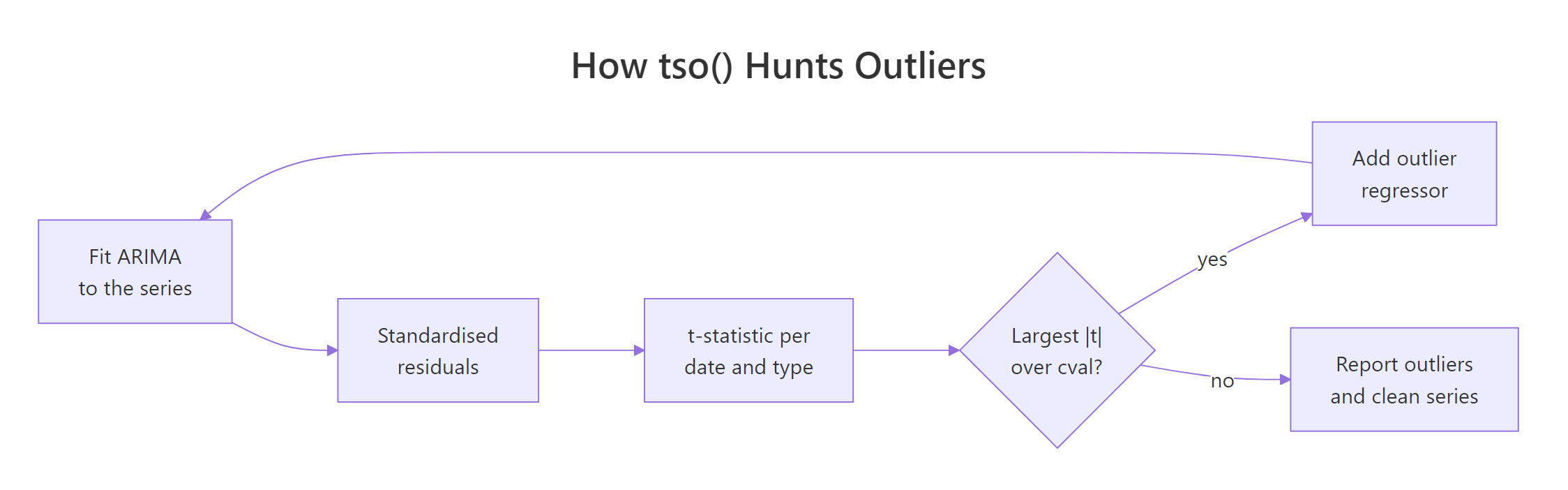
Figure 3: The tso() loop: fit, test every date, absorb the worst offender, refit.
Walking through the loop in plain English:
- Fit an ARIMA model to the series. ARIMA is the standard model for describing how a series relates to its own recent past.
tso()picks the model automatically, so you do not have to choose orders. - Take the residuals and standardise them, which puts them on a comparable scale.
- Test every date against every shape. For each date and each anomaly type in
types, compute a t-statistic asking "if an anomaly of this shape started here, how big would it be relative to its own uncertainty?" - Compare the largest t-statistic to
cval, the critical value. If nothing clears the bar, stop. - Absorb the winner. Add that anomaly as a regressor column, refit the ARIMA model with it included, and go back to step 2.
The loop matters. Once a genuine anomaly is absorbed into the model, the residuals shrink, and the next round tests against a cleaner baseline. That is how the procedure separates one large real event from the smaller distortions it creates around itself.
Enough theory. Point it at the Nile.
Two anomalies, and the first one is the century-old story the z-score could not see. LS at time 1899 is a level shift: a permanent drop of 242 units, arriving exactly when construction of the Aswan Low Dam began. The second, AO at 1913, is a one-off low year that returns to normal immediately.
Compare that to the z-score's answer of "nothing unusual here". Same data, same century, and the difference is entirely in what the two methods were looking for.
You can also print the whole fitted object to see the model underneath.
This is an ordinary regression printout with the two outliers as predictors. intercept is 1097.75, which is that pre-break average you computed by hand earlier. LS29 has a coefficient of -242.23 and a standard error of 26.78, so the step is estimated nine times more precisely than its own size. ARIMA(0,0,0) means that once the level shift is accounted for, nothing is left to model, no autoregressive terms and no moving-average terms. The step was the structure.
types argument is c("AO", "LS", "TC"), which is what this call uses explicitly. Innovational outliers are excluded because on an annual, non-seasonal series like the Nile they are hard to distinguish from additive outliers, and adding types you cannot identify slows the search and invites false positives.Try it: Ask tso() to look for additive outliers only. If the level shift is genuinely a step and not a spike, restricting the search should make it vanish from the results.
Click to reveal solution
Explanation: The 1899 level shift has disappeared entirely, because a permanent step simply is not the shape types = "AO" searches for. The 1913 spike survives with a slightly different coefficient (-405.4 instead of -399.5), because it is now being measured against a model that never learned about the step. The lesson is blunt: a detector only ever finds shapes you asked it for, so leaving LS out of types means you will never be told about a permanent change no matter how large it is.
How do you read the tso() output and repair the series?
The outliers table has five columns and every one of them earns its place. Using the Nile result as the worked example:
| Column | Value in row 1 | What it means |
|---|---|---|
type |
LS |
The shape: additive outlier, level shift or temporary change |
ind |
29 |
The position in the series, counting from 1 |
time |
1899 |
The calendar label for that position |
coefhat |
-242.2289 |
The size of the effect, in the series' own units |
tstat |
-9.045372 |
The size divided by its own standard error |
coefhat is the column you quote to another human being. It says the Nile lost 242 units of annual flow, permanently, and it is measured in the same units as the data. tstat is the column the algorithm uses to decide. It is just the coefficient divided by its standard error, which you can verify from the printout above.
That reproduces tstat exactly. The number means the estimated step is 9 standard errors away from zero, so the probability of seeing a step that clean in noise alone is vanishingly small. Anything past roughly 3 is already strong evidence, so 9 is not a borderline call.
So how does an anomaly actually enter the model? As a plain column of numbers. outliers.effects() builds those columns for you, and looking at them makes the whole method concrete.
outliers.effects() takes the outliers table and the series length, and returns one column per anomaly. We wrap it in a data frame with the actual years so the rows are readable. Now look at the two columns.
LS_1899 is 0 before 1899 and 1 from 1899 onward, forever. It is a switch that flips on and stays on, which is precisely what "permanent step" means as arithmetic. AO_1913 is 0 everywhere except the single year 1913. It is a pulse.
Multiply each column by its coefhat and add them to the intercept and you have reconstructed the model. That is the entire trick: an anomaly type is just a differently shaped column of ones and zeros. The level shift is a step function, the additive outlier is a pulse, and a temporary change would be a pulse that decays geometrically.
Which brings us to the practical payoff. If you know the shape and the size, you can subtract the anomaly back out. tso() has already done it and stored the result in yadj.
The two lines agree perfectly for 1897 and 1898, because the level shift had not started yet. From 1899 they diverge by roughly 242 units every single year, which is exactly coefhat. The adjusted series answers a specific hypothetical: what would the flow have looked like if the dam had never been built?
yadj to model, not to report. The level shift was real, so a "repaired" Nile is a fiction. It is useful as a modelling input, because a series without the step is easier to forecast, but never hand it to someone as if it were the measurement.The last dial is cval, the critical value a t-statistic has to beat. tso() picks a default from the series length, roughly 3 for a series of 100 points. Lower it and you catch more.
Dropping cval from about 3 to 2.8 takes the count from 2 to 5. The 1899 level shift is still there and now looks stronger, with a t-statistic of -10.9, because a better-specified model gives a cleaner estimate. But the three new additive outliers have t-statistics of 2.80, 2.93 and 2.95, all sitting barely over the new bar. Those are the definition of marginal calls.
cval because you have a reason (a short series, a known-noisy sensor), never because the result looks more interesting.Try it: Go the other way. Tighten cval to 4 so only overwhelming evidence survives, and see which of the two original anomalies is strong enough to make the cut.
Click to reveal solution
Explanation: At cval = 4 the table is empty, which is surprising at first because the 1899 shift had a t-statistic of -9.05, comfortably past 4. The catch is that cval gates every stage of the loop, including the first pass over the raw residuals before any anomaly has been absorbed. At that stage no single candidate clears 4, so the loop stops before it ever gets to refit, and nothing is reported. The practical lesson: cval is not a post-hoc filter you can crank up to keep only the best findings. It changes the search itself, so raising it too far can hide the very anomaly that would have dominated the results.
How does the anomalize pipeline flag anomalies in a data frame?
tso() is a specialist. It takes one ts object, fits a model, and tells you the shape of what it found. That is exactly what you want when you have one important series and a question about it.
It is not what you want when you have 400 dashboards refreshing every morning. For that you want speed, a tidy data frame in and out, and the ability to run every series at once. That is anomalize.

Figure 4: The three anomalize verbs and the columns each one adds.
The pipeline is three verbs, and each one adds columns to your data frame rather than replacing it. Start with time_decompose().
Alongside the table, R prints four status messages telling you it converted the tibble, picked date as the index, and chose frequency = 7 days and trend = 91 days. Those two choices are what frequency = "auto" and trend = "auto" resolved to: a weekly season and a quarter-long window for estimating the trend. The function inspects the spacing of your dates to pick them, which is why it needs a real Date column.
The method = "stl" argument means Seasonal-Trend decomposition using Loess, a standard technique that splits a series into three additive parts. Read the row for 2017-01-01: the observed count was 643, the season contribution was -2,078 (a New Year's Day Sunday, deep in the weekend trough), the trend was 2,474, and the remainder was 246.
Those three parts are not approximations. They add back up exactly.
Identical, to the unit. The decomposition is a lossless rewrite of the data into three interpretable pieces, and that is what makes the rest of the pipeline work.
Now the second verb, which draws the limits.
Three new columns appear. remainder_l1 and remainder_l2 are the lower and upper limits, here -3,323 and 3,310, and they are the same on every row because the IQR method computes one pair of limits for the whole series. anomaly is a plain "Yes" or "No" telling you whether that row's remainder fell outside them.
Look at 2017-01-02: a remainder of -1,659 is large, but it sits inside the fence, so the verdict is No. That is the pipeline working correctly. A quiet day right after New Year is unusual against the raw average and completely ordinary against its own season.
Nineteen days out of 425, about 4.5 percent. That is a plausible number for real operational data, and a very different answer from the z-score's three.
The third verb translates the limits back into the units your reader thinks in.
time_recompose() adds the season and trend back onto the remainder limits, producing recomposed_l1 and recomposed_l2: the range of counts that would have been normal on that specific date. Unlike the remainder limits, these move every row.
That movement is the whole point. On 2017-01-12 the normal range was 199 to 6,832 and the count was 0, below the floor. On 2018-02-07 the normal range was 5,216 to 11,849 and the count was 11,924, just above the ceiling. A fixed threshold could never call both of those correctly, because 11,924 is a fine number in February and would be extraordinary in January.
Notice how many of the flagged days show observed of exactly 0. Let us check that directly.
Seven of the nine outage days are caught, against zero out of nine for the z-score. The two misses are worth understanding rather than glossing over: they fall on days whose seasonal expectation was already very low (a weekend in the trough), so a count of zero was not far enough below the floor to clear the limit. That is a genuine limitation of a purely statistical detector, and it is why a zero-count rule and an anomaly detector are complementary rather than redundant.
Finally, the package draws the whole thing for you.
Figure 5: The grey band is the recomposed normal range, which widens and narrows with the weekly cycle. Red dots are the flagged days.
time_recomposed = TRUE draws the grey band from recomposed_l1 and recomposed_l2. The band narrows at weekends and widens midweek, and it drifts upward as the trend grows. That moving band is the visual version of everything this section has covered.
ts, convert it first with something like tibble(date = ..., value = as.numeric(my_ts)). Passing a ts straight in will fail, because the pipeline reads the date column to work out the frequency.Try it: The IQR limits come from the remainder's own quartiles. Compute the 25th and 75th percentiles of lub_dec$remainder and the distance between them, then compare that distance to the limits of -3,323 and 3,310 you saw above.
Click to reveal solution
Explanation: The middle half of the remainders spans just 948 units, from -480 to 467, yet the limits sit out at roughly plus and minus 3,320. That is about 3.5 IQRs on either side, which is where alpha comes in: anomalize scales the fence by 0.15 / alpha, so alpha = 0.05 gives a factor of 3. Two useful facts fall out of this. The limits depend only on the middle of the distribution, so a handful of huge outliers cannot drag them outward, and alpha is a direct multiplier on the fence width rather than a p-value.
When should you use GESD instead of IQR?
anomalize() accepts a second method, "gesd", and the choice between the two is the most consequential tuning decision in the pipeline. Both answer the same question, "which remainders are too far out?", but they go about it in opposite ways.
IQR computes its limits once. It reads the quartiles of all 425 remainders, sets a single fence from them, then applies that fence to every row. Fast, and completely deterministic.
GESD works iteratively. It finds the most extreme remainder, tests whether it is more extreme than you would expect from that many draws of a normal distribution, removes it, recomputes the mean and standard deviation without it, and repeats. GESD stands for Generalised Extreme Studentised Deviate, and it is the test Twitter's anomaly-detection work popularised.
That iteration solves a specific problem called masking. If your series has six catastrophic days, those six inflate the standard deviation so much that a mildly bad seventh day looks perfectly normal by comparison. The big outliers mask the smaller ones. GESD removes them one at a time, so the standard deviation shrinks as it goes and the smaller offenders become visible.
Thirty flagged instead of nineteen, on identical input. The obvious question is whether GESD found different days or simply more of them.
The intersection is 19, which is every single day IQR found. GESD's set strictly contains IQR's set, and adds 11 more. This is masking made visible: those 11 days were always mildly unusual, but the huge zero-download days were inflating the spread enough to hide them. Peel the big ones off and the moderate ones surface.
Scan the extra dates and they make sense. 2017-12-25, 2017-12-26 and 2017-12-29 are Christmas week. 2017-04-26, 04-27 and 04-29 cluster in a single week. These are real events of a smaller size, not random noise.
Here is how the two compare in practice.
| IQR | GESD | |
|---|---|---|
| How limits are set | Once, from the quartiles | Iteratively, one point removed per round |
| Resists masking | No | Yes |
| Speed | Very fast | Slower, but fine to a few thousand points |
| Typical result | Fewer, more extreme flags | More flags, including moderate ones |
| Best for | Monitoring at scale, alerting on the worst | Investigation, forensic passes, clustered events |
Whichever method you pick, alpha controls how permissive it is. Sweeping it makes the sensitivity concrete.
The loop reruns anomalize() four times and counts the flags. Halving alpha from 0.05 to 0.025 cuts the count from 19 to 4; doubling it to 0.10 raises it to 44. alpha moves the answer by an order of magnitude across a perfectly reasonable range, which means it is not a setting you can leave to chance.
The mechanism is the formula from the last exercise: the IQR fence is scaled by 0.15 / alpha. At alpha = 0.05 that is a factor of 3, and at alpha = 0.20 it drops to 0.75, a fence narrower than the interquartile range itself.
One thing to keep straight: alpha does not mean the same thing in both methods. Under IQR it is only that multiplier, with no probability attached to it. Under GESD it is a real significance level, the false-positive rate the test accepts on each round of its search. The same number therefore is not directly comparable across the two, so tune it separately per method rather than carrying a value across.
alpha that recovers those events without burying you in extras. Choosing it by "that looks about right" bakes your expectations into the detector.The other dial is max_anoms, and it works differently from alpha in a way that catches people out.
alpha is held at 0.20 throughout, so the statistical test is identical in all three runs and would flag 84 days if left alone. Only max_anoms changes. At 0.01 you get 4 flags, which is 1 percent of 425. At 0.05 you get 21, which is 5 percent.
max_anoms is not a test. It is a hard ceiling expressed as a fraction of the series, and it keeps only the most extreme candidates up to that count.
max_anoms times the row count, that is the ceiling talking, not the data. Raise it and rerun before you trust the number.Try it: Run GESD with a much stricter alpha of 0.01 and see whether it still beats IQR's 19. This tells you whether GESD's extra finds come from being iterative or just from being permissive.
Click to reveal solution
Explanation: Even at alpha = 0.01, five times stricter than the IQR run, GESD still flags 27 days against IQR's 19. So the extra detections are not the result of a looser threshold, they come from the iterative procedure genuinely un-masking days that IQR's single fixed fence could never reach. If you need to be confident you have not missed a moderate event, that is a real argument for GESD, and it costs you only compute time.
How do you scan many series for anomalies at once?
Everything so far has run on one series. Real monitoring is never one series. It is every product line, every region, every endpoint, and if your detector needs a for loop and a list of results to stitch back together, you will not run it daily.
The pipeline handles this without any new functions, because the verbs respect dplyr grouping. tidyverse_cran_downloads arrives already grouped by package, so all 15 series can go through in a single pass.
That is 6,375 rows across 15 series, decomposed, tested and recomposed by the same three lines you ran on one package, in about a second. Each package gets its own seasonal pattern, its own trend and its own limits, because the grouping is respected at every step. lubridate still shows the 19 anomalies you found earlier, which confirms the grouped run and the single run agree.
The ranking is the actual deliverable. broom has 34 anomalous days and glue has 3, so if you can only investigate two series this morning, you now know which two.
Plotting a grouped result faceted by series lets you eyeball a whole fleet at once. Fifteen panels is too many to read, so take four.
Figure 6: Four packages, one pipeline, one chart. Each panel has its own band because each series was decomposed separately.
Each panel carries its own grey band, sized to that package's own weekly pattern and trend. A shared y-axis and a shared threshold would have made ggplot2, the busiest of the four, swamp the others entirely.
Try it: Anomalies come in two flavours: counts above the ceiling and counts below the floor. Using four_anom, count only the spikes for each package, meaning rows where observed is above recomposed_l2.
Click to reveal solution
Explanation: Compare these to the totals from the grouped run: ggplot2 had 21 anomalies but only 1 is a spike, so 20 are dips. tidyr had 22 with 7 spikes. Across all four packages, dips outnumber spikes heavily, which fits CRAN download data where the failure mode is a mirror going offline rather than a sudden surge. Splitting flags by direction takes about ten seconds and usually tells you more about root cause than the raw count does, so make it a habit.
Which engine should you choose for your problem?
You now have two working detectors, so the question is when to reach for which. The honest way to answer it is to show each one failing at the other's job.
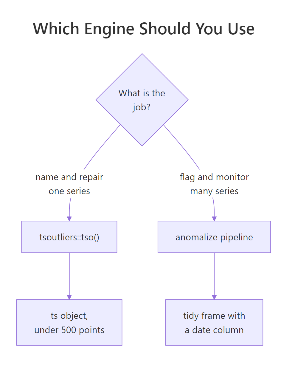
Figure 7: Choosing between tso() and the anomalize pipeline.
Start with the failure that surprises people. Take the Nile, the series whose level shift tso() identified with a t-statistic of -9.05, and push it through the anomalize pipeline.
One row in the output, and it says No a hundred times. The anomalize pipeline finds nothing in the Nile. Not a weak signal, not a marginal call: zero flagged points in the series containing one of the most studied structural breaks in statistics.
This is not a bug, and understanding why is the most useful idea in this whole tutorial. time_decompose() splits the series into season, trend and remainder. A level shift is, mathematically, a change in the level, so STL absorbs it into the trend component. The trend line simply steps down in 1899 and carries on. By the time anomalize() looks at the remainder, the shift has already been explained away, and what is left really is unremarkable noise.
tso() finds it because it tests for a step explicitly, as a named hypothesis, rather than looking at leftovers.Now the reverse failure. tso() refits an ARIMA model on every iteration of its loop, so cost grows quickly with series length and with the number of types you search. On 100 annual points it is instant. On 6,375 daily rows across 15 groups, where the pipeline finished in about a second, tso() would need a separate call per series and a noticeable wait for each. It also returns ind, a position, so you have to map results back to dates yourself.
Here is the decision, laid out.
tsoutliers::tso() |
anomalize pipeline |
|
|---|---|---|
| Input | A ts object |
A data frame with a date column |
| Question it answers | What kind of event was this, and how big? | Which rows are unusual right now? |
| Names the shape | Yes: AO, LS, TC, IO, SLS | No, just Yes or No |
| Finds level shifts | Yes, that is its speciality | No, decomposition absorbs them |
| Gives a repaired series | Yes, via yadj |
No |
| Many series at once | One call per series | Native, respects group_by() |
| Comfortable size | Up to a few hundred points | Thousands of rows across many groups |
| Main dial | cval |
alpha and max_anoms |
The practical rule is short. Use anomalize to find out that something happened, and tso() to find out what it was. They are complementary, not competing, and the Complete Example below runs them exactly that way.
timetk package offers plot_anomaly_diagnostics() and tk_anomaly_diagnostics(), which wrap the same decompose-then-IQR logic with a slightly different interface. If your project already leans on timetk, those functions save you a dependency. The concepts in this tutorial transfer directly.Try it: Confirm the null result above rather than taking it on trust. Filter nile_anom to the flagged rows and look at what comes back.
Click to reveal solution
Explanation: A tibble with 0 rows, and R helpfully lists the columns that would have been there. This is the output worth remembering, because it is what a silent failure looks like in practice. Nothing errored, nothing warned, and a pipeline that returns an empty set reads exactly like "all clear". Whenever a detector reports zero anomalies on data you believe is eventful, check whether the shape you care about is one the method can represent at all.
Complete Example: an end-to-end anomaly audit
Time to put both engines together on a series we have not touched yet. broom had the most anomalies of the 15 packages, 34 of them, so it makes a good subject. The workflow is the one you would run in production: screen broadly, classify narrowly, then repair.
Stage 1: screen the whole series with anomalize.
Thirty-four flagged days out of 425, exactly matching what the grouped run reported earlier. That is our candidate list.
Stage 2: split the candidates by direction and timing.
A clean 17-17 split between dips and spikes. The weekday breakdown of the dips is the interesting part: 9 of the 17 land on a Friday or Saturday. Remember that the pipeline has already removed the weekly season, so this is not "weekends are quiet". It is a genuine tendency for whatever breaks to break at the end of the week, which is precisely the kind of lead an operations team can act on.
Stage 3: look at the worst offenders.
All three are zero-count days, and all three had a floor of at least 2,843. Two of them, 2018-02-09 and 2018-02-23, are exactly two weeks apart. That pattern is worth naming properly, which is Stage 4.
Stage 4: classify the shape with tso().
Three things are happening in that block, so take them one at a time.
We cut a 46-day window around the events, because tso() is happiest on short series and we already know from Stage 3 where to look. ts(win$count, frequency = 7) wraps the counts as a weekly-seasonal time series, which is what tso() expects. Then, because tso() reports ind as a position rather than a date, we index back into win$date to recover real calendar dates, which is the small piece of glue that makes the output shareable.
The verdict: both events are temporary changes, not additive outliers. That distinction is the payoff of the whole exercise. An additive outlier would mean one broken day followed by an immediate return to normal. A TC means the effect decayed back over several days, so downloads did not simply resume the next morning, they climbed back gradually. The effect sizes, -4,664 and -4,440, say each event cost about 4,500 downloads at its worst.
Two temporary changes of near-identical size, exactly 14 days apart, is the signature of a recurring biweekly failure rather than two unrelated incidents. Two events are not proof of a schedule, but the pattern is specific enough to take to whoever runs the mirror and check against their job logs.
Stage 5: recover what the numbers should have been.
yadj estimates what each day would have been without the event. The gap closes as you read down: 4,664 lost on the 9th, 3,265 on the 10th, 2,286 on the 11th, and by the 13th the series is nearly back. That decay is the "temporary" in temporary change, made concrete.
Add the five gaps and the incident cost roughly 13,000 downloads. That is a number you can take to a status page, and you got there by screening with anomalize, classifying with tso(), and reading the repair off yadj.
Practice Exercises
These combine several ideas from the tutorial. Each uses my_-prefixed variable names so nothing you built above gets overwritten.
Exercise 1: Audit a package and split the flags by direction
Run the full three-verb pipeline on the dplyr download series with method = "iqr" and alpha = 0.05. Report how many days were flagged in total, and how many of those were dips, meaning observed fell below recomposed_l1.
Click to reveal solution
Explanation: Sixteen anomalies, eleven of them dips. The 16 matches the grouped run from the multi-series section exactly, which is the check worth making: a single-series pipeline and a grouped one must agree, because the grouping only changes how rows are batched, never how limits are computed. The dip-heavy split, 11 down against 5 up, is the same pattern the four-package exercise showed, and it points at CRAN mirror availability rather than at bursts of interest.
Exercise 2: Plant a level shift and recover it
Simulate a series of 80 points where the first 40 are drawn from a normal distribution with mean 100 and standard deviation 4, and the last 40 from mean 128 with the same standard deviation. Use set.seed(2026). Run tso() on it, then check the estimated shift size against the difference between the two halves' actual means.
Click to reveal solution
Explanation: tso() recovers the planted shift precisely. It reports a single LS at position 41, which is the exact index where the distribution changed, with a coefficient of 27.65 against a true shift of 28. The segment means, 100 and 127, differ by 27, so the estimate is right to within a fraction of one standard deviation. The t-statistic of 32.8 is enormous because the shift is seven times the noise level. Worth noting what is absent: no spurious additive outliers were reported around the break, even though types included them, because the loop absorbed the step first and left nothing for the other shapes to explain.
Exercise 3: Compare the two detection methods on a new series
Run the pipeline on the tidyquant series using method = "gesd" with alpha = 0.05, and report how many days were flagged and how many of those were spikes (observed above recomposed_l2). Then build a small data frame comparing IQR and GESD flag counts on the lub_dec object from earlier.
Click to reveal solution
Explanation: Two results worth sitting with. First, tidyquant breaks the pattern every other series showed: 15 of its 20 anomalies are spikes rather than dips. tidyquant is a finance package, so bursts of interest around market events are a plausible driver, and it is a reminder that "anomalies are usually dips" was a fact about CRAN infrastructure, not a law. Second, the comparison confirms the section-6 finding in one table: GESD flags 30 where IQR flags 19 on identical input. Running both and looking at the difference costs almost nothing and tells you how much masking your series has.
Frequently Asked Questions
What is the difference between an outlier and an anomaly in a time series?
In everyday use they are the same word. In time series work the useful distinction is that an outlier is a value far from the rest of the data, while an anomaly is a value far from what the series predicted for that moment. The Nile shows why that matters: its level shift is a genuine anomaly and contains no outliers at all, which is why a z-score reported zero findings on it.
Should I remove anomalies from my data before forecasting?
It depends entirely on the shape. Remove an additive outlier, because a mistyped number or a logging glitch carries no information about the future. Never remove a level shift, because it is real and permanent, and deleting it teaches your model to forecast a world that no longer exists. Use tso() to name the shape before you decide, and remember that yadj gives you the repaired series only when repair is the right call.
Does anomalize work on a ts object?
No. time_decompose() reads a date or date-time column to work out the frequency and trend windows, so it needs a data frame, not a ts. Convert first with tibble(date = your_dates, value = as.numeric(your_ts)). Going the other way, tso() needs a ts object, which you build with ts(df$value, frequency = 7) for daily data with a weekly cycle or frequency = 12 for monthly data.
How much data do I need before anomaly detection is reliable?
For anomalize you want at least two full seasonal cycles so STL can separate season from trend, which means about two weeks for daily data with a weekly cycle and about two years for monthly data. For tso() the constraint is different: the default cval is derived from the series length, and with fewer than about 50 points the procedure has little power, so genuine anomalies go unreported.
Why does anomalize flag more days than I expected?
Check alpha first. Under IQR it is a direct multiplier on the fence width rather than a p-value, with a factor of 0.15 / alpha; under GESD it is a genuine significance level, so the same value behaves differently in the two methods. Then check whether your flagged count is sitting at exactly max_anoms times your row count, which means the cap truncated the result rather than the data producing it. Finally, GESD normally flags more than IQR on the same series, so switching methods alone can change the number substantially.
Can I detect anomalies in real time as new data arrives?
Both tools here are retrospective: they look at a whole series at once and decide which points were unusual. For streaming use, the standard pattern is to rerun the pipeline on a rolling window (say the last 90 days) each time a batch arrives, and treat only the newest rows' flags as alerts. Be aware that a point near the end of a window has less context on one side, so it is judged less reliably than a point in the middle.
Is anomalize still maintained?
The package is on CRAN and works, and the same decompose-then-test approach now also ships inside timetk as tk_anomaly_diagnostics() and plot_anomaly_diagnostics(). If you are starting a new project that already uses timetk, those functions save you a dependency. Everything in this tutorial about decomposition, IQR, GESD and alpha transfers to them directly.
Summary
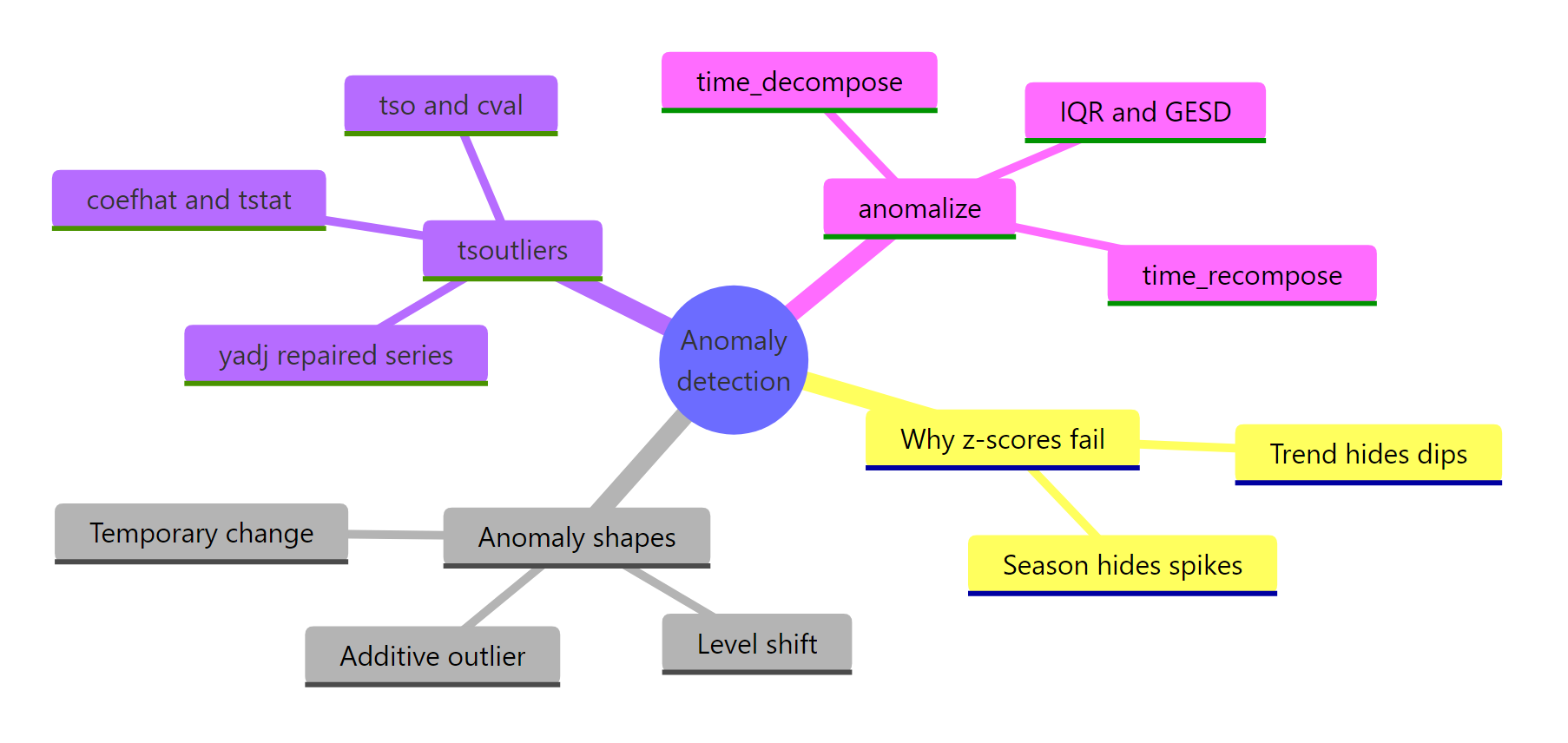
Figure 8: Everything this tutorial covered, in one map.
| Question | Tool | The line of code |
|---|---|---|
| Is a z-score enough? | No, it ignores trend and season | (x - mean(x)) / sd(x) finds 0 anomalies in the Nile |
| What shape is this anomaly? | tsoutliers |
tso(y, types = c("AO", "LS", "TC")) |
| How big was it, in real units? | The coefhat column |
fit$outliers$coefhat |
| What would the series have been without it? | The adjusted series | fit$yadj |
| How sensitive is the search? | The critical value | tso(y, cval = 2.8) |
| Which rows of my data frame are unusual? | anomalize |
time_decompose() then anomalize() then time_recompose() |
| What counted as normal on that date? | The recomposed bounds | recomposed_l1 and recomposed_l2 |
| Am I missing moderate events? | Switch methods | anomalize(remainder, method = "gesd") |
| How do I loosen or tighten it? | alpha, capped by max_anoms |
alpha = 0.05 gives an IQR factor of 3 |
| How do I run 400 series? | Group the data frame | group_by(series) before time_decompose() |
The four ideas worth carrying away:
- Judge each point against its own moment, not the series average. Both packages do this. It is the entire difference between them and a z-score.
- Name the shape before you decide what to do. A spike gets fixed, a level shift gets modelled, and treating one as the other corrupts your data or your forecast.
- A detector only finds shapes it can represent. anomalize returns zero anomalies for the Nile, silently, because STL folds a level shift into the trend.
- Screen with
anomalize, classify withtso(). They answer different questions and the workflow that uses both beats either one alone.
References
- Chen, C. and Liu, L.-M. (1993). Joint Estimation of Model Parameters and Outlier Effects in Time Series. Journal of the American Statistical Association, 88(421), 284-297. The paper
tso()implements; the package PDF below restates the procedure and the outlier filters in full. Link - López-de-Lacalle, J. tsoutliers: Detection of Outliers in Time Series. CRAN package page and reference manual. Link
tso()function reference, with every argument includingtypes,cval,maxit.iloopandtsmethod. Link- Dancho, M. and Vaughan, D. anomalize: Tidy Anomaly Detection. CRAN package page. Link
- Business Science. Anomaly Detection Using Tidy and Anomalize, the package announcement explaining the IQR and GESD lineage. Link
- Rosner, B. Percentage Points for a Generalized ESD Many-Outlier Procedure. Technometrics, 25(2), 165-172 (1983). The source of the GESD method; the NIST handbook page below works through the test statistic and critical values step by step. Link
- Cleveland, R. B., Cleveland, W. S., McRae, J. E. and Terpenning, I. STL: A Seasonal-Trend Decomposition Procedure Based on Loess. Journal of Official Statistics, 6(1), 3-73 (1990). The decomposition
time_decompose()uses. Link - Hyndman, R. J. and Athanasopoulos, G. Forecasting: Principles and Practice, 3rd edition. Chapter 3: Time series decomposition. Link
forecast::tsoutliers()reference, the lightweight interpolation-based detector that inspired the IQR method. Link
Continue Learning
- Time Series Decomposition in R: the STL machinery behind
time_decompose(), covered properly: how season, trend and remainder are estimated and what the window arguments actually control. - Test Stationarity in R: a level shift is one way a series stops being stationary, and these tests tell you whether the break you found is the only one.
- Moving Averages in R: the smoothing ideas that trend estimation is built on, and a lighter-weight way to spot a series drifting away from its own recent behaviour.