Variational Bayes in R: Fast Approximate Inference
Variational Bayes (VB) is a way to approximate a Bayesian posterior by turning inference into optimization: you pick a simple, easy-to-handle distribution, then slide and stretch it until it fits the true posterior as closely as possible. Unlike MCMC, which draws thousands of samples and can be slow, VB never samples. It tunes a handful of numbers and stops. That trade, a fast answer that is close rather than a slow answer that is exact, is what makes variational Bayes the workhorse for large models. This post builds VB from scratch in R so you can see exactly what it optimizes and where it goes wrong, then shows you how to run it with one argument in a real package.
What is variational Bayes, and why is it faster than MCMC?
If you have read the MCMC tutorial, you know the sampling recipe: propose a move, accept or reject it, repeat until a long chain of draws traces out the posterior. It works, but it can be slow, and on a big model you may wait minutes or hours for the chain to settle. Variational Bayes attacks the same problem from a completely different direction. Instead of collecting samples, it proposes a simple distribution and then adjusts that distribution's parameters until it matches the posterior as well as it can. Sampling becomes optimization.
The cleanest way to meet the idea is to start where we can check the answer perfectly. Suppose you measure a quantity 40 times with known noise, put a Normal prior on its mean, and ask for the posterior of that mean. For this Normal-with-a-Normal-prior setup the posterior is itself a Normal distribution with a formula, so we know the exact answer in advance. That gives us a target to compare against.
That block simulated the data and then applied the textbook Normal-Normal update. A precision is just one over a variance, and the update is clean in that currency: the posterior precision is the prior precision plus the data precision, and the posterior mean is a precision-weighted blend of the prior mean and the data mean. The posterior for our quantity is a Normal centered at 4.878 with a standard deviation of 0.316. Hold onto those two numbers. They are the truth that VB will try to recover.
Now the variational part. We declare that our approximation, written $q$, is a Normal distribution with an unknown mean m and standard deviation s. VB scores every candidate (m, s) with a single objective called the ELBO (we unpack it in the next section) and picks the pair that scores highest. Higher ELBO means the candidate Normal sits closer to the posterior. We hand that objective to R's optim() and let it climb.
Read what just happened. We started optim() at a mean of 0 and a spread of 1, and it searched over (m, s) to push the ELBO as high as it could. The mean it settled on, 4.878, and the spread, 0.316, are exactly the closed-form posterior from the first block. VB recovered the true posterior without a single sample, purely by optimizing. The whole fit takes a fraction of a second.

Figure 1: Variational Bayes reframes inference as optimization. Choose a simple family, then push the ELBO uphill until it stops rising, and read off the fitted distribution as your approximate posterior.
Here the match was perfect for one reason: the true posterior was a Normal, and we searched a family of Normals, so the best member of the family was the posterior itself. In almost every real problem the posterior is not so tidy, and the best Normal is only a good approximation, not an exact copy. That gap is the entire story of variational Bayes, and the rest of this post is about seeing it clearly and knowing when it hurts.
Try it: Rerun the exact posterior with 400 measurements instead of 40 and confirm the posterior standard deviation shrinks as data accumulates. Because this posterior is Normal, the ELBO fit would land on the very same numbers.
Click to reveal solution
With 400 points the posterior standard deviation drops from 0.316 to 0.100. More data means a tighter posterior, and VB tracks it because the exact posterior stays inside the Normal family it searches.
What are the ELBO and KL divergence, in plain terms?
We waved at the ELBO above. Now let us define it, because it is the quantity every variational method maximizes. Two ideas do all the work, and both have a plain-language reading before any symbols.
The first is a way to measure how different two distributions are. The KL divergence from your approximation $q$ to the true posterior $p$ is a number that is zero when they are identical and grows as they drift apart. Think of it as a distance from $q$ to the posterior, though it is not symmetric. VB wants this as small as possible.
The second is the ELBO, short for evidence lower bound. It is a score you can actually compute for any candidate $q$, and it is tied to the KL divergence by a clean identity.
The ELBO is the expected log joint density minus the expected log of your approximation:
$$\text{ELBO}(q) = \mathbb{E}_{q}\!\left[\log p(x, \theta)\right] - \mathbb{E}_{q}\!\left[\log q(\theta)\right]$$
Where:
- $\theta$ is the parameter you want to infer, and $x$ is the observed data
- $p(x, \theta)$ is the joint density, the likelihood times the prior, which you can always write down
- $q(\theta)$ is your simple approximating distribution
- $\mathbb{E}_{q}$ means an average taken over $\theta$ drawn from $q$
The reason the ELBO matters is this identity, which splits the log evidence into two pieces:
$$\log p(x) = \text{ELBO}(q) + \mathrm{KL}\!\left(q(\theta)\,\|\,p(\theta \mid x)\right)$$
The log evidence $\log p(x)$ on the left is a fixed number: it does not depend on $q$. So when you raise the ELBO, the KL divergence must fall by the same amount, because the two always add up to that fixed total. Maximizing the ELBO is therefore the same as minimizing the distance from $q$ to the posterior, which is exactly what we want. The name "lower bound" comes from the fact that KL is never negative, so the ELBO can never exceed the log evidence.
A tiny discrete example makes the identity concrete. Imagine the posterior lives over just three possible values, and we have an unnormalized score for each. The evidence is the sum of those scores.
Look at the last two numbers. The ELBO of our rough guess is 2.221, and the log evidence minus the KL divergence is also 2.221. The identity holds exactly. The ELBO fell short of the log evidence (2.303) by precisely the KL gap (0.081). If you set $q$ equal to the true posterior, the KL gap closes to zero and the ELBO rises to meet the log evidence, which is the best any approximation can do.
Try it: Nudge the approximation closer to the truth and confirm its ELBO rises while its KL divergence falls.
Click to reveal solution
The closer approximation scores a higher ELBO (2.2947 versus 2.221) and a smaller KL (0.0079 versus 0.081). Climbing the ELBO always means shrinking the distance to the posterior.
What is the mean-field approximation, and when does it fail?
So far our approximation had one unknown. Real models have many parameters, and their posteriors tangle those parameters together through correlations. The mean-field approximation is the assumption that makes VB tractable at scale: it treats the parameters as independent, so the joint approximation factors into a separate simple distribution for each one.
$$q(\theta) = \prod_{j} q_j(\theta_j)$$
With that factorization, there is a beautifully simple algorithm called coordinate ascent variational inference (CAVI). You update one factor at a time, holding the others fixed, using the rule below, and you cycle through the factors until the ELBO stops rising.
$$\log q_j^\star(\theta_j) = \mathbb{E}_{q_{-j}}\!\left[\log p(x, \theta)\right] + \text{const}$$
Where $q_{-j}$ means all the factors except the one you are currently updating. Each update is a one-factor optimization, which is why mean-field VB is fast even with thousands of parameters.
To watch CAVI work and to expose its famous weakness, we need a posterior with real correlation. A Bayesian linear regression with an intercept and a slope is perfect: when the predictor is not centered, the posterior for the intercept and the slope is a tilted, correlated Gaussian. Because the model is simple we can also compute that posterior exactly, so once again we have a truth to check against.
That block built the exact posterior for the intercept b0 and the slope b1. The posterior mean is roughly (4.301, 1.247), and the two coefficients are strongly anti-correlated, with a correlation of -0.867. That negative correlation is intuitive: with an uncentered predictor, a line that tilts up more steeply must start lower to still pass through the cloud of points, so a larger slope forces a smaller intercept. Mean-field VB will ignore exactly this link.
Now run CAVI. Each factor is a Normal; the mean-field math says every factor's variance is fixed at one over the corresponding diagonal of the precision matrix, and the means are updated by the coordinate rule until they settle. We track the ELBO so we can watch it climb.
Two things happened. First, the CAVI means converged to (4.301, 1.247), the exact posterior mean from the previous block. Mean-field VB nailed the location. Second, the ELBO climbed at every step, from -16.563 up to -3.840, and flattened out by iteration 10, which is how you know CAVI has converged. The ELBO values are negative here only because we dropped an additive constant; what matters is that the objective rose monotonically and levelled off.
The catch is in the spread. Compare the standard deviations CAVI produced against the true posterior standard deviations.
VB reports a standard deviation that is only 0.498 of the true one for both coefficients, so it is about half as wide as it should be. That is not a coincidence: for a two-parameter Gaussian the shrinkage factor is exactly $\sqrt{1 - \rho^2}$, and with a correlation of -0.867 that works out to 0.498, matching the ratios to three decimals. The stronger the correlation the mean-field factorization throws away, the more overconfident VB becomes. A picture makes the failure obvious.
The plot draws the true 95% posterior region against the VB one over a scatter of posterior samples. The true region is a long, tilted ellipse: the anti-correlation shows up as the downhill lean. The VB region is a smaller, upright ellipse that captures the center but sits entirely inside the truth and lines up with the axes, blind to the tilt. It is a correct location with a wrong sense of uncertainty.
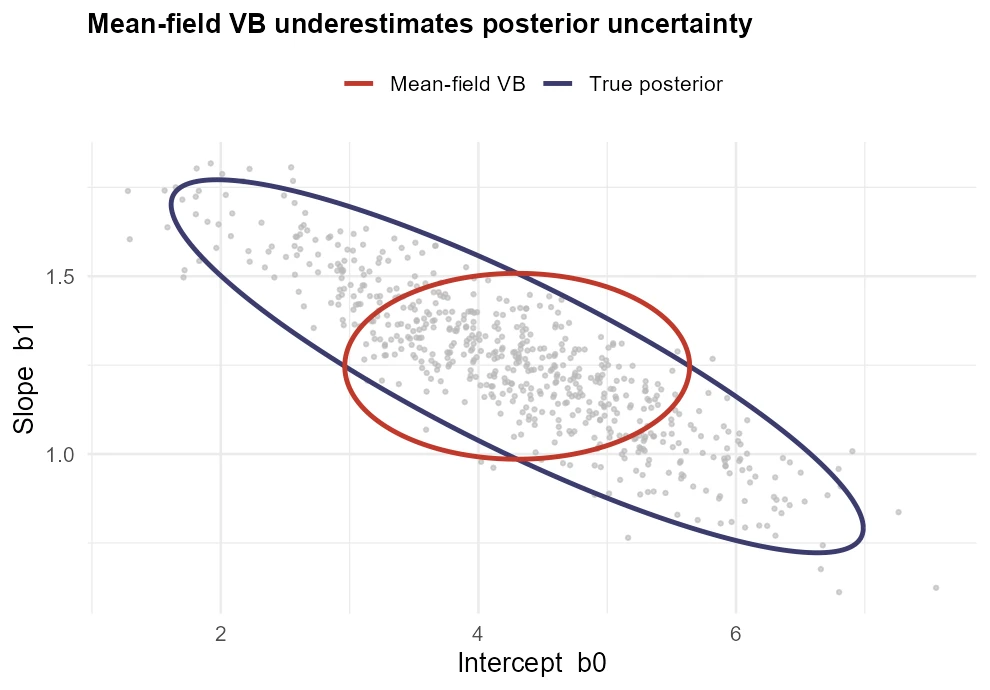
Figure 2: Mean-field VB (red) matches the posterior centre but is narrower and axis-aligned, so it misses the true correlation captured by the full posterior (navy).
Try it: Center the predictor by subtracting its mean, rebuild the posterior, and check what happens to the correlation and the underestimation.
Click to reveal solution
Centering drives the correlation to 0, and the underestimation factor becomes 1, meaning VB now reports the exact posterior spread. This is a genuinely useful trick: centering (and more generally reparameterizing to reduce correlation) makes mean-field VB far more accurate.
How do you run variational Bayes with a real R package?
Building CAVI by hand is the best way to understand VB, but for everyday work you reach for a package that does it for any model you can write. The rstanarm package fits a full range of Bayesian regressions and lets you switch from MCMC to variational Bayes by changing a single argument: algorithm = "meanfield". Under the hood it runs a general-purpose variational method called ADVI, which applies the same optimize-the-ELBO idea to models far more complex than our hand-built example.
rstanarm installed. Everything above this section runs directly on the page.library(rstanarm)
options(mc.cores = 1)
# Variational Bayes: one argument switches sampling off
fit_vb <- stan_glm(mpg ~ wt, data = mtcars,
algorithm = "meanfield", seed = 123, refresh = 0)
# The usual full MCMC fit, for comparison
fit_mc <- stan_glm(mpg ~ wt, data = mtcars,
chains = 4, iter = 2000, seed = 123, refresh = 0)
coef(fit_vb) # VB point estimates
posterior_interval(fit_vb, prob = 0.90) # VB 90% intervals
coef(fit_mc) # MCMC point estimates
posterior_interval(fit_mc, prob = 0.90) # MCMC 90% intervalsA representative run gives the comparison below (your VB digits will move slightly from run to run, which we explain in a moment).
| Coefficient | VB estimate | VB 90% interval | MCMC estimate | MCMC 90% interval |
|---|---|---|---|---|
| Intercept | 37.4 | [34.1, 40.8] | 37.2 | [34.1, 40.4] |
| wt (slope) | -5.37 | [-6.4, -4.4] | -5.31 | [-6.3, -4.4] |
Read the table against what we learned by hand. The VB point estimates land almost exactly on the MCMC ones (37.4 versus 37.2 for the intercept, -5.37 versus -5.31 for the slope), and it finished faster. That is the reliable half of variational Bayes: it gets the location right, quickly. The intervals are in the same ballpark but should be read as an approximation, not a final answer.
Two honest caveats come with the package. First, ADVI optimizes with a dose of randomness, so rerun the fit and the last digits of every number shift; a single VB run is one noisy estimate, not a fixed truth. Second, on this toy model both methods finish in under a second, so the speed argument looks weak here. The real payoff arrives at scale: when a model has thousands of parameters or millions of rows, MCMC can run for hours while VB returns in seconds or minutes. That is when variational Bayes earns its place.
If you outgrow rstanarm, the same switch exists elsewhere. The brms package accepts algorithm = "meanfield" or "fullrank" for the same ADVI engine, and Stan's newer "pathfinder" method gives a fast variational-style approximation that often initializes MCMC well. All of them optimize an ELBO.
So when should you pick VB over MCMC? The rule of thumb below captures it.
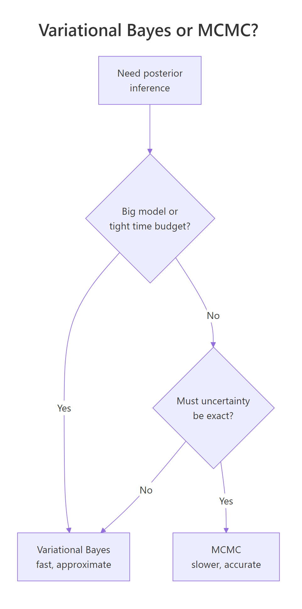
Figure 3: A quick rule for choosing between variational Bayes and MCMC based on model size and how exact your uncertainty needs to be.
Reach for variational Bayes when the model is large or you need an answer fast and can tolerate approximate uncertainty, for example during exploration and prototyping, or as a warm start for MCMC. Stay with MCMC when the model is small enough to sample comfortably and you need credible intervals you can quote with confidence.
Try it: VB reported the wt coefficient with a posterior mean near -5.38 and a posterior standard deviation near 0.63. Turn those two summaries into a 90% credible interval and the probability that the slope is negative.
Click to reveal solution
The 90% credible interval runs from -6.416 to -4.344, and the probability the slope is negative rounds to 1. Because a mean-field marginal is Gaussian, every summary you want comes from qnorm and pnorm. Just remember the width is the optimistic VB estimate, not the wider truth.
A complete example: wrap variational Bayes into one function
To pull the from-scratch pieces together, here is the whole mean-field regression fit collapsed into one reusable function. It takes a predictor, a response, and the known noise level, and returns the VB means alongside the VB and true standard deviations so you can always see the overconfidence at a glance.
The function recovered the coefficients (an intercept near 1.23 and a slope near 0.88, close to the true 1 and 0.8), and once again the vb_sd column is well below the true_sd column. Even on fresh data with a different design, the pattern holds: mean-field VB is trustworthy for the center and optimistic about the spread. Keeping the true standard deviation beside the VB one, whenever you can afford to compute it, is a good habit for calibrating how much to inflate a VB interval.
vb_sd sit below true_sd on every fit trains your eye to widen a variational interval before you quote it.Practice Exercises
These combine the ideas above. Each starter block runs as written so you can iterate; the solution follows.
Exercise 1: Match VB to a closed-form posterior
You observe 12 measurements with known noise sig_known = 1.5 and a Normal(0, 3) prior on the mean. Compute the closed-form Normal-Normal posterior mean and standard deviation, then fit a Gaussian by maximizing the ELBO (as in section one), and confirm the two agree.
Click to reveal solution
The closed-form and VB answers match to three decimals (mean 2.637, standard deviation 0.429), because a single-parameter Normal posterior is inside the Gaussian family VB searches. With one parameter there is no correlation to lose, so VB is exact.
Exercise 2: Quantify the mean-field underestimation
You are given a two-parameter Gaussian posterior with standard deviations 1 and 0.5 and a correlation of 0.9. Without any data, apply the mean-field rule (each variance is one over the matching diagonal of the precision matrix) and report the factor by which VB shrinks each standard deviation. Confirm it equals $\sqrt{1 - 0.9^2}$.
Click to reveal solution
Both coefficients shrink to 0.4359 of their true spread, exactly $\sqrt{1 - 0.9^2}$. At a correlation of 0.9, mean-field VB reports intervals less than half as wide as they should be, a strong warning against trusting VB uncertainty when parameters are tightly linked.
FAQ
Is variational Bayes always faster than MCMC?
Usually, and by a wide margin on large models, but not always on tiny ones. VB solves an optimization problem, which often converges in far fewer steps than a sampler needs to mix. On a small model like a two-variable regression, though, MCMC already finishes in a moment, so the speed gap is small. The advantage grows with model size and data volume.
Does variational Bayes give the wrong answer?
It gives an approximate answer. Point estimates (posterior means) are typically very close to the truth, as every example here showed. The uncertainty is where it slips: mean-field VB systematically underestimates variance and ignores correlations, so its credible intervals are too narrow. It is right about where the parameters are and overconfident about how sure you should be.
How is variational Bayes different from the Laplace approximation?
Both approximate the posterior with a simpler distribution, but they fit it differently. The Laplace approximation puts a Gaussian at the posterior mode using the curvature there, a purely local fit. Variational Bayes chooses its approximation by minimizing KL divergence over the whole distribution, a global fit. VB also handles non-Gaussian factors and mean-field factorizations that Laplace does not.
Can I trust a VB credible interval?
Treat it as a lower bound on the real width. If the interval already excludes a value you care about (like zero) by a wide margin, the conclusion is probably safe, since the true interval is wider but centered the same place. If a decision hinges on the exact interval, verify with a short MCMC run before you quote it.
Which R packages do variational Bayes?
For applied regression, rstanarm and brms both expose ADVI through algorithm = "meanfield" or "fullrank". Stan itself offers "pathfinder" for a fast variational-style start. For custom models you can code CAVI by hand, exactly as this post did, whenever the updates have a closed form.
Summary
| Idea | What to remember |
|---|---|
| Core trade | VB swaps MCMC sampling for optimization: fast and approximate instead of slow and exact |
| The objective | Maximize the ELBO, which is equivalent to minimizing the KL divergence from your approximation to the posterior |
| Mean-field | Assume the parameters are independent so the approximation factorizes; enables the CAVI algorithm |
| The failure mode | Mean-field ignores correlations, so it underestimates posterior spread by a factor of $\sqrt{1-\rho^2}$ in the two-parameter case |
| What VB gets right | Point estimates (posterior means) are usually excellent; the location is reliable |
| Practical fix | Centering or reparameterizing to reduce correlation makes mean-field VB much more accurate |
| In practice | Switch on VB with algorithm = "meanfield" in rstanarm or brms; verify uncertainty against MCMC when it matters |
References
- Blei, D. M., Kucukelbir, A., & McAuliffe, J. D. (2017). Variational Inference: A Review for Statisticians. Journal of the American Statistical Association. Link The definitive modern survey; derives the ELBO and CAVI in full.
- Kucukelbir, A., Tran, D., Ranganath, R., Gelman, A., & Blei, D. M. (2017). Automatic Differentiation Variational Inference. Journal of Machine Learning Research. Link The paper behind the
algorithm = "meanfield"engine used in this post. - Stan Development Team. Stan Reference Manual: Variational Inference. Link How Stan implements ADVI and what its options mean.
- Stan Development Team. rstanarm: Bayesian applied regression modeling via Stan. Link Package docs for the applied regression fits shown here.
- Stan Development Team. vb: Variational inference reference for rstan. Link The lower-level
vb()entry point if you write your own Stan model. - Dablander, F. (2019). A brief primer on Variational Inference. Link A gentle, R-based walk through the same ideas, good for a second pass.
Continue Learning
- MCMC in R: Build Metropolis-Hastings From Scratch provides the sampling counterpart to this post. Read both to see the two great families of Bayesian computation side by side.
- Bayesian Linear Regression in R fits the same intercept-and-slope model with full MCMC and shows how to read a posterior you can trust.
- The Bayesian Workflow in R puts approximate and exact inference in context: when to prototype fast and when to slow down and check.