Bayesian Nonparametrics in R: Dirichlet Process Clustering
Dirichlet process clustering is a Bayesian method that groups data into clusters without making you choose the number of clusters in advance. It treats the cluster count as something to learn from the data, so the number of groups can grow as more data arrives.
Most clustering tools ask you a question you often cannot answer: "How many clusters are there?" A Dirichlet process turns that question around and lets the data answer it. In this tutorial you will build the idea up from scratch, run every piece of it right here in your browser, and finish by fitting the same model with a ready-made package. We use base R throughout the hands-on parts, so there is nothing to install to follow along.
Why does ordinary clustering make you guess the number of clusters?
Popular clustering methods like k-means need one thing before they can start: the number of clusters, usually written as k. On a real dataset you rarely know k ahead of time. That is often the whole reason you are clustering. To see why guessing hurts, let us make some data where we secretly know the answer, then watch a standard method react to different guesses.
We will create 120 points that fall into three tight groups, centered far apart at -6, 0, and 6. Because we built them, we know the truth is three clusters of 40 points each. Run the block to make the data and confirm its shape.
The output confirms 120 points split evenly into groups A, B, and C, and the first few values sit near -6 as expected. A quick histogram makes the three groups obvious to the eye.
You can see three separate humps, so a good clustering method should recover three groups. Now let us hand k-means the wrong number of clusters and see what it does. We ask it for 2 clusters, then for 5.
With k set to 2, k-means merges two real groups into one blob of 80 points. With k set to 5, it chops the data into five pieces even though only three exist. In both runs it returned exactly as many clusters as we asked for, whether or not that number was right. It never questioned the guess.
Try it: Rerun k-means on the same data, but this time ask for 3 clusters and read off the three sizes. Change the centers value in the starter, then run it. You should get three sizes close to 40, 40, 40.
Click to reveal solution
Explanation: With the right k, k-means recovers the three groups perfectly (nstart = 25 just runs several random starts and keeps the best). The catch is that you had to know the answer was 3 to get here. A Dirichlet process removes that catch.
What is a Dirichlet process, in plain words?
A Dirichlet process is a recipe for splitting points into groups where the number of groups is not fixed ahead of time. Instead of deciding k, you set one dial called the concentration parameter, written $\alpha$, that controls how readily new groups appear. The clusters themselves are an outcome of the process, not an input to it.
The friendliest way to picture it is the Chinese restaurant process. Imagine a restaurant with endless tables. Customers arrive one at a time. Each new customer either joins a table that already has people (and prefers busier tables) or sits at a fresh empty table. The tables become your clusters, and the customers become your data points.
The rule for where a customer sits is simple. A new point joins an existing cluster with probability proportional to how many points are already there, and starts a brand new cluster with probability proportional to $\alpha$.
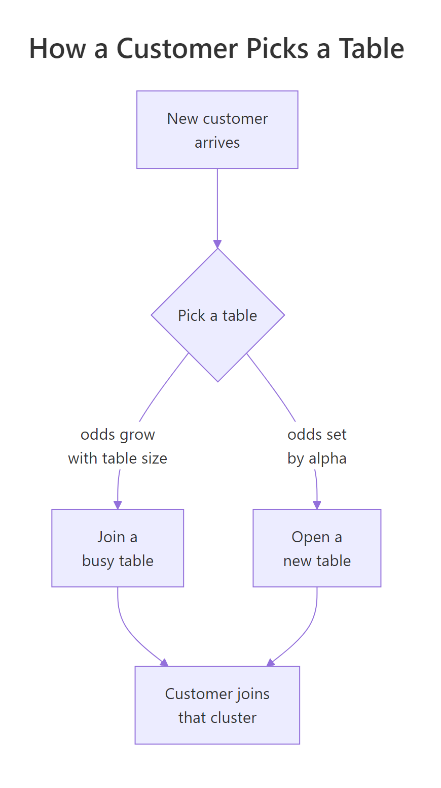
Figure 1: How a new point joins a busy cluster or starts a new one under the Chinese restaurant process.
We can write the seating rule as two probabilities. For the $i$-th customer arriving at a restaurant that already has some occupied tables:
$$P(\text{join cluster } k) = \frac{n_k}{i - 1 + \alpha}, \qquad P(\text{start a new cluster}) = \frac{\alpha}{i - 1 + \alpha}$$
Where:
- $n_k$ = the number of points already sitting in cluster $k$
- $i - 1$ = how many points have been seated so far (everyone except the arriving point)
- $\alpha$ = the concentration parameter, the dial that controls new clusters
The denominator is $i - 1 + \alpha$ because the $i$-th customer sees $i - 1$ people already seated, and this matches the i - 1 + alpha you are about to see in the code (there i is the current customer and the argument n is just the total number of customers to seat).
Notice the "rich get richer" effect: a table with more people is more likely to attract the next customer, because $n_k$ is bigger. Let us turn that rule into code. The function below seats n customers one by one and returns the table number each one chose.
Twenty customers walked in and, without anyone setting the number, they settled into four tables. One table drew a crowd of 15, one seated 3, and two tables held a single diner each. The line probs <- c(counts, alpha) / (i - 1 + alpha) is the seating rule in action: it lists the odds for every current table (using their headcounts) followed by the odds of opening a new one (using $\alpha$), then sample() picks one.
Try it: Seat 30 customers instead of 20 with the same $\alpha$, then count how many tables opened. Change n in the starter and run it. Bigger crowds tend to open a few more tables.
Click to reveal solution
Explanation: Thirty customers filled three tables this time, with one clear favorite holding 21 people. The exact count shifts with the random seed, which is the point: the number of clusters is itself uncertain and depends on the data.
How does the concentration parameter alpha control the number of clusters?
The concentration parameter $\alpha$ is the one dial you set, so it pays to build a feel for it. A small $\alpha$ makes the process reluctant to open new tables, so you get a few big clusters. A large $\alpha$ makes it eager, so you get many small ones. Let us measure this directly by simulating the restaurant many times at each setting and averaging how many tables appear.
The helper below runs crp() reps times for a given $\alpha$ and reports the average number of tables for 100 customers.
The pattern is clear and steady. At $\alpha = 0.5$ the same 100 customers form about 3 clusters on average, while at $\alpha = 10$ they spread across nearly 24. Raising $\alpha$ raises the expected number of clusters in a smooth, predictable way. This is the knob you tune when you want the model to be more or less willing to split data into new groups.
Try it: Push $\alpha$ up to 20 and see how many clusters 100 customers form on average. Change the alpha argument and run it. Expect a number in the mid-30s.
Click to reveal solution
Explanation: At $\alpha = 20$ the same 100 points scatter into about 36 clusters on average. A large concentration parameter makes the process split hair-thin, which is usually too many groups to be useful, so $\alpha$ is often kept small or learned from the data.
How does stick-breaking turn alpha into cluster weights?
The Chinese restaurant process describes how points get assigned. There is a second, equivalent view that describes the cluster sizes directly, called stick-breaking. It is worth seeing because it makes the role of $\alpha$ visual and is the construction most software uses under the hood.
Picture a stick of length 1 that represents all the probability. You break off a random fraction for the first cluster, then break off a fraction of what remains for the second cluster, and so on. Each break uses a random fraction drawn from a Beta distribution that depends on $\alpha$. The pieces are the cluster weights, and they always shrink as you go.
$$\beta_k \sim \text{Beta}(1, \alpha), \qquad \pi_k = \beta_k \prod_{j < k} (1 - \beta_j)$$
Where:
- $\beta_k$ = the fraction we snap off at step $k$
- $\pi_k$ = the final weight (relative size) of cluster $k$
- $\prod_{j < k}(1 - \beta_j)$ = the length of stick still left before step $k$
If the math looks heavy, skip it: the code below is the whole idea, and its output tells the story. It breaks the stick ten times for $\alpha = 2$ and prints the resulting weights.
The first few clusters grab the biggest slices (0.262, 0.224, and so on) and later clusters get crumbs. The weights add up to 0.999 rather than exactly 1 because we stopped after ten breaks and a sliver of stick is still unbroken. In a full Dirichlet process you would keep breaking forever, but in practice a handful of clusters soak up almost all the weight.
Try it: Break the stick with a much smaller $\alpha$ of 0.5 and watch how lopsided the weights become. Change the alpha argument and run it. The first piece should dominate.
Click to reveal solution
Explanation: With $\alpha = 0.5$ the first cluster takes almost 80 percent of the weight and the rest is nearly nothing. Small $\alpha$ concentrates points into a few dominant clusters, which is exactly what the restaurant simulation showed from the other direction.
How do you actually cluster data with a Dirichlet process mixture?
So far we have seen how a Dirichlet process invents clusters, but not how it clusters real numbers. The missing piece is a model for what a cluster looks like. We attach a bell curve (a Normal distribution) to each cluster, so a cluster is just a group of points sharing a center. This combination, a Dirichlet process choosing clusters plus a Normal describing each one, is called a Dirichlet process mixture model, and it is the workhorse for clustering when k is unknown.
To fit it, we sweep through the points many times. On each pass we take one point out and re-seat it using the same restaurant rule, except now the odds are weighted by how well the point fits each cluster's bell curve. A point that lands near a cluster's center is likely to join it; a point far from every cluster is more likely to open a new one. Repeating this thousands of times lets the cluster assignments settle down. This procedure is a collapsed Gibbs sampler.
We need one ingredient: a score for how well a point fits a cluster. Because we assume a known spread inside clusters and a Normal prior on each cluster's center, the score has a clean closed form. It is the height of a Normal curve, centered on the cluster's updated mean, evaluated at the point.
$$p(x_i \mid \text{cluster } k) = \mathcal{N}\!\left(x_i \;\middle|\; m_k,\; s_k^2 + \sigma^2\right)$$
Where:
- $x_i$ = the point we are scoring
- $m_k$ = the cluster's updated center after seeing its current members
- $s_k^2$ = how unsure we are about that center
- $\sigma^2$ = the assumed spread of points around a center
If you would rather not read the formula, the function below is all you need. It returns a fit score for a point against a cluster's current members, and it handles the empty case (a brand new cluster) by falling back to the prior.
The score of 0.4881 is just the height of the fitted Normal curve at the point, and higher means a better fit. With that scorer in hand, the sampler itself is a loop. For each point it removes the point, scores every existing cluster (weighted by cluster size) plus the option of a new cluster (weighted by $\alpha$), then draws an assignment from those odds.
Now the payoff. We run the sampler on our original data x, the one we know has three groups, without ever telling it that number. We use a small $\alpha$ of 0.3, assume a modest within-cluster spread, and let it sweep 150 times. Then we look at how many clusters it settled on and compare its groups to the truth.
The model found three clusters on its own, and it recovered the grouping exactly: every A point landed in one cluster, every B in another, every C in a third, with no mixing. The table(tail(...)) line shows that across the last 50 sweeps the sampler most often reported 3 clusters (39 out of 50 times), occasionally reporting 4 or 5. We can also color the raw points by their inferred cluster to see the clean split.
Try it: Raise $\alpha$ from 0.3 to 5 and rerun the sampler on the same x. Change the alpha argument and run it. A bigger $\alpha$ pushes the model to split the same data into many more clusters.
Click to reveal solution
Explanation: With $\alpha = 5$ the same three-group data gets carved into roughly 9 clusters, because a large concentration parameter rewards opening new tables. This is the concrete danger of setting $\alpha$ too high, and why it is worth choosing it carefully or learning it from the data.
How do you run this with a package instead of coding it yourself?
Coding the sampler by hand is the best way to understand it, but for real work you will reach for a tested package. The dirichletprocess package fits the same Dirichlet process mixture in a few lines and handles the sampling for you. Because it relies on compiled internals, it does not run in the in-page runner, so treat the next block as code to run in your own R or RStudio session.
install.packages("dirichletprocess"), then run the code in RStudio. The output shown below was produced by running it locally on the same kind of data.We rebuild the three-group data, standardize it (the package expects roughly standardized input), and fit a Gaussian Dirichlet process mixture with 1000 sampling steps. Then we ask how many clusters it found and check them against the truth.
library(dirichletprocess)

# same three groups as before, then standardized
set.seed(101)
xp  <- c(rnorm(40, -6, 0.5), rnorm(40, 0, 0.5), rnorm(40, 6, 0.5))
grp <- rep(c("A", "B", "C"), each = 40)
yp  <- as.numeric(scale(xp))

set.seed(2024)
dp <- DirichletProcessGaussian(yp)
dp <- Fit(dp, 1000, progressBar = FALSE)

dp$numberClusters
#> [1] 3
table(true = grp, cluster = dp$clusterLabels)
#>     cluster
#> true  1  2  3
#>    A 40  0  0
#>    B  0  0 40
#>    C  0 40  0
The package reached the same conclusion our hand-built sampler did: three clusters, one per real group, with a perfect split. The difference is that it took three lines instead of a page of code, and it comes with well-tested samplers and support for more cluster shapes than a single bell curve.
Practice Exercises
These two problems combine the pieces you just built. Each has a runnable starter and a hidden solution with the expected output. Use fresh variable names so you do not overwrite the tutorial's objects.
Exercise 1: Predict the cluster count from alpha
Use the avg_tables() helper to estimate how many clusters 50 customers form on average when $\alpha = 3$, over 300 simulated restaurants. Set the seed to 55 first so your answer is reproducible.
Click to reveal solution
Explanation: Fifty customers at $\alpha = 3$ form about 9 clusters on average. This reuses the same simulation from the alpha section, now as a quick planning tool: pick $\alpha$, and you can predict roughly how many groups to expect before you ever touch real data.
Exercise 2: Let the sampler discover two clusters
Make a new dataset with just two well-separated groups (50 points near -4 and 50 near 4), then run dp_gibbs() on it and check whether the model discovers two clusters. Use sigma2 = 0.5, tau2 = 25, and 120 sweeps. Confirm the result with a cross-tabulation against the true groups.
Click to reveal solution
Explanation: Handed two-group data, the same sampler settles on two clusters (38 of the last 40 sweeps) and splits them cleanly: all left points in one cluster, all right points in the other. The exact same code that found three groups earlier found two here, with no change to the number of clusters. That is the whole promise of the method.
FAQ
Is Dirichlet process clustering just a fancy k-means? No. k-means fixes the number of clusters up front and only moves centers around. A Dirichlet process treats the number of clusters as unknown and lets it grow with the data, so it answers a question k-means cannot even ask.
Does it always recover the true number of clusters? It recovers a range, not a single number. The model reports a distribution over how many clusters fit the data, which is more honest than a point estimate. When groups are well separated it concentrates tightly on the right count, as you saw; when they overlap, the range is wider.
What value of alpha should I use? Start small, around 0.5 to 1, since large values invent too many tiny clusters. Better still, many packages can learn $\alpha$ from the data by placing a prior on it, so you do not have to guess. The simulations here show why the choice matters: $\alpha$ directly sets how eager the model is to split.
Do I need to scale my data first? For the dirichletprocess package, yes. Its default settings assume roughly standardized input, so call scale() before fitting. Our from-scratch sampler used a wide prior instead, which is another way to stay insensitive to the data's scale.
Why is it called nonparametric if there are still parameters? "Nonparametric" here means the number of parameters is not fixed in advance. Each new cluster adds its own center, so the model can use more parameters as more data arrives. It is unbounded flexibility, not the absence of parameters.
Summary
You now have both the intuition and the working code for clustering when the number of clusters is unknown. The table below recaps the moving parts.
| Concept | What it does | Where it appeared here |
|---|---|---|
| Chinese restaurant process | Seats points into clusters, favoring busy ones | The crp() simulation |
| Concentration parameter alpha | Sets how eagerly new clusters open | The alpha-vs-clusters table |
| Stick-breaking | Turns alpha into shrinking cluster weights | The stick_breaking() weights |
| Dirichlet process mixture | Clusters real numbers with a Normal per group | The dp_gibbs() sampler |
| dirichletprocess package | Fits the same model in a few tested lines | The run-locally block |
The mind map below ties the pieces together: one problem, three views of the same process, a single tuning dial, then two ways to run it in R.
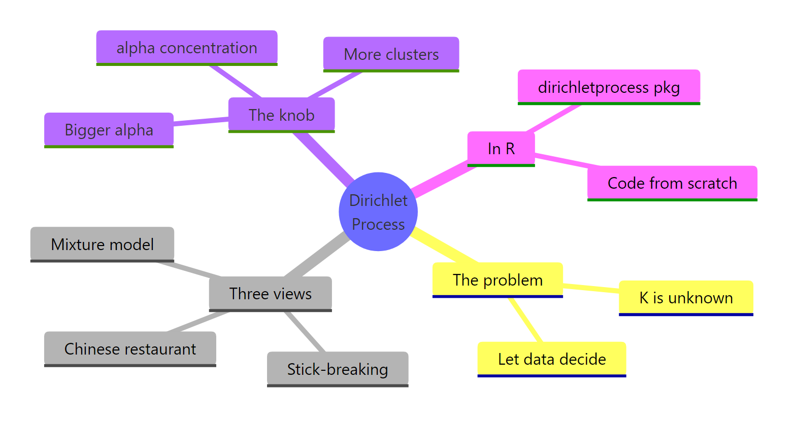
Figure 2: The Dirichlet process at a glance: the problem it solves, its three views, its single tuning dial, then two ways to run it in R.
The big idea to carry away: a Dirichlet process replaces the awkward question "how many clusters?" with a single tuning dial and lets the data supply the count. That makes it a natural fit for exploratory work where you genuinely do not know the structure ahead of time.
References
- dirichletprocess package on CRAN. Link - the package used in the last section; install page and reference manual.
- Ross, G. J. and Markwick, D. (2018). dirichletprocess: An R Package for Fitting Complex Bayesian Nonparametric Models. Link - the paper behind the package, walking through its models and API.
- dirichletprocess package vignette (PDF). Link - worked examples of fitting Dirichlet process mixtures with the package.
- Neal, R. M. (2000). Markov Chain Sampling Methods for Dirichlet Process Mixture Models. Link - the classic reference for the collapsed Gibbs sampler this post builds by hand.
- Rasmussen, C. E. (2000). The Infinite Gaussian Mixture Model. Link - the paper that popularized the Dirichlet process Gaussian mixture for clustering.
- Teh, Y. W. (2010). Dirichlet Process. Encyclopedia of Machine Learning. Link - a compact, readable definition of the process and its Chinese-restaurant and stick-breaking views.
- CRAN Task View: Bayesian Inference. Link - a curated index of R packages for Bayesian work, including nonparametric ones.
- Chinese restaurant process (overview). Link - a plain-language reference for the seating rule that drives the clustering.
Continue Learning
- Grid Approximation in R: compute Bayesian posteriors directly on a grid, a gentle first step into Bayesian computation before samplers.
- Gaussian Mixture Models in R: the fixed-k cousin of this model, where you do choose the number of clusters in advance.
- Gibbs Sampling in R: a closer look at the sampling engine that powers the clustering sampler you built here.