RStan vs brms vs BayesFactor: Which to Use in R?
Three R packages get recommended for Bayesian work, and they are not interchangeable. For most applied regression, reach for brms: one formula and it writes the model for you. When you need a model no formula can express, drop to RStan and write it by hand. When your question is "which hypothesis does the data support?" rather than "what is the fitted model?", use BayesFactor. This guide shows what each one actually gives you back, with runnable code, so you can pick the right tool the first time.
Which Bayesian package should you use in R?
You have a Bayesian question and three well-known packages. Which one do you open? The whole decision fits in one small function you can run right now. It asks two yes/no questions and hands back a package name.
Here is what the function did. It checked the two flags in priority order. If you need a Bayes factor, nothing else matters and it returns BayesFactor. If you are building a custom model, it returns RStan. Otherwise it falls through to brms, which is the right answer for the large majority of real analyses.
The three test calls map the three most common situations to their packages. A routine regression goes to brms, a hypothesis test goes to BayesFactor, and a hand-built model goes to RStan. That ordering is the core idea of this whole post.
Try it: You are building a fully custom model by hand, not a standard regression. Call recommend_package() with the right argument so it returns "RStan".
Click to reveal solution
Explanation: Setting custom_model = TRUE skips the brms default and returns RStan, the package you use when you write the model yourself.
Posterior or Bayes factor: what do you actually get back?
Before you can choose, you need to see the one difference that splits the three packages into two camps. It is about what comes out the other end.
brms and RStan both return a posterior: a whole probability distribution for every parameter, given your data. It answers "given what I saw, what values are plausible for this slope, and how sure am I?" BayesFactor returns a Bayes factor: a single number saying how much the data shifted the balance between two hypotheses. It answers "did the data favor one story over another, and by how much?"
To make "a posterior is a whole distribution" concrete, here is one you can compute in base R with no special package. Imagine you saw 7 successes in 10 trials and want to know the success rate. We lay out a grid of candidate rates, score each by how well it explains 7 out of 10, and normalise.
Read the output as a shape, not a single answer. Each of the 11 numbers is the probability that the true rate sits near that grid point. The mass piles up around 0.6 to 0.8 and the average lands at 0.667. That spread is the posterior, and it is exactly the kind of object brms and RStan give you for every parameter in a real model.
A Bayes factor throws that shape away on purpose and returns one number instead. That is not worse, it is a different question. You will see it in action later with the BayesFactor package.
Try it: Suppose you saw only 3 successes in 10 trials instead of 7. Recompute the posterior mean. It should move well below 0.5.
Click to reveal solution
Explanation: Fewer successes pull the whole distribution toward smaller rates, so the mean drops from 0.667 to 0.333. The posterior moved as a shape, not just as a single point.
How does brms turn a formula into a model?
brms is the package most people should reach for, so it is worth seeing why it feels so easy. You describe the model with the same formula syntax you already use for lm() and glm(), and brms handles the rest. A complete Bayesian linear regression is one line:
brm(mpg ~ wt, data = mtcars)
Behind that line, brms does two things you would otherwise do by hand. First, it chooses sensible default priors for you. You can inspect them without fitting anything using get_prior(), which needs no model compilation and runs right here.
library(brms)
get_prior(mpg ~ wt, data = mtcars)
#>                    prior     class coef group resp dpar nlpar lb ub tag       source
#>                   (flat)         b                                           default
#>                   (flat)         b   wt                                 (vectorized)
#>  student_t(3, 19.2, 5.4) Intercept                                           default
#>     student_t(3, 0, 5.4)     sigma                             0             default
That table is brms telling you its plan. The slope for wt gets a flat (uninformative) prior, the intercept and the residual standard deviation get weakly informative Student-t priors scaled to your data. You can override any row, but for a first fit the defaults are reasonable.
Second, brms writes the actual model in Stan's own language and compiles it. You can see the exact program it generates with make_stancode(mpg ~ wt, data = mtcars). This is the code brms produces from that one formula:
// generated with brms 2.23.0
data {
  int<lower=1> N;  // total number of observations
  vector[N] Y;  // response variable
  int<lower=1> K;  // number of population-level effects
  matrix[N, K] X;  // population-level design matrix
  int<lower=1> Kc;  // number of population-level effects after centering
}
parameters {
  vector[Kc] b;  // regression coefficients
  real Intercept;  // temporary intercept for centered predictors
  real<lower=0> sigma;  // dispersion parameter
}
model {
  // priors
  target += student_t_lpdf(Intercept | 3, 19.2, 5.4);
  target += student_t_lpdf(sigma | 3, 0, 5.4);
  // likelihood
  target += normal_id_glm_lpdf(Y | Xc, Intercept, b, sigma);
}
That is dozens of lines of careful Stan code, written for you from a single formula. When you actually run brm(), it compiles this, samples from it, and summary(fit) prints each parameter's posterior mean, error, 95% credible interval, and convergence diagnostics. You get a full Bayesian regression without ever opening the Stan file.
Try it: Inspect the default priors for a model with two predictors, mpg ~ wt + hp. How many rows does the prior table gain?
# Call get_prior() on mpg ~ wt + hp and read the extra coefficient row.
# get_prior(mpg ~ wt + hp, data = mtcars)
Click to reveal solution
get_prior(mpg ~ wt + hp, data = mtcars)
#>                    prior     class coef group resp dpar nlpar lb ub tag       source
#>                   (flat)         b                                           default
#>                   (flat)         b   hp                                 (vectorized)
#>                   (flat)         b   wt                                 (vectorized)
#>  student_t(3, 19.2, 5.4) Intercept                                           default
#>     student_t(3, 0, 5.4)     sigma                             0             default
Explanation: Adding hp gives the table one more coefficient row (b for hp). brms assigns each predictor its own prior automatically, so growing the model never means hand-writing more prior code.
When is raw Stan with RStan worth the extra effort?
If brms is so convenient, when would you ever step down to RStan? The answer is control. brms can only express models its formula syntax supports. When your model has a structure no formula captures, a custom likelihood, a hard parameter constraint, an unusual hierarchy, you write the Stan program yourself and drive it with RStan.
Here is a hand-written Stan program for the same simple regression. Notice that you declare every variable, prior, and the likelihood explicitly:
// A simple linear regression, written by hand for RStan
data {
  int<lower=0> N;        // number of observations
  vector[N] x;           // predictor (weight)
  vector[N] y;           // outcome (mpg)
}
parameters {
  real alpha;            // intercept
  real beta;             // slope
  real<lower=0> sigma;   // residual standard deviation
}
model {
  beta ~ normal(0, 10);                  // prior on the slope
  y ~ normal(alpha + beta * x, sigma);   // likelihood
}
With RStan you save that program, then hand it your data as a named list whose names match the data block above. Building that list is plain R, and you can run it now to see the structure Stan expects:
From there the RStan workflow is three calls in your local R session: mod <- rstan::stan_model("model.stan") compiles the program, fit <- rstan::sampling(mod, data = stan_data) runs the sampler, and print(fit) shows the posterior summaries. The rstan::stan() function bundles all three into one call. The result is the same kind of posterior brms gives you, but you controlled every line that produced it.
Try it: Rebuild the data list with a standardized weight (mean 0, standard deviation 1). Standardizing predictors often helps Stan's sampler.
Click to reveal solution
Explanation: scale() centers and scales the predictor, so the new x has mean 0 and standard deviation 1. Feeding standardized predictors to Stan usually makes the sampler converge faster.
What can BayesFactor do that brms and RStan cannot?
BayesFactor answers a question the other two do not answer directly: how strongly does the data favor one hypothesis over another? It compares two models, usually a null and an alternative, and returns their evidence ratio. That ratio is the Bayes factor.
$$\text{BF}_{10} = \frac{p(\text{data} \mid H_1)}{p(\text{data} \mid H_0)}$$
Where:
- $\text{BF}_{10}$ = the Bayes factor for the alternative $H_1$ against the null $H_0$
- $p(\text{data} \mid H_1)$ = how well the alternative predicted the data, averaged over its priors
- $p(\text{data} \mid H_0)$ = how well the null predicted the data
A $\text{BF}_{10}$ of 20 means the data are 20 times more likely under the alternative than the null. Values above about 10 are usually called strong evidence, values near 1 mean the data barely moved your beliefs.
You can build a rough Bayes factor yourself in base R from two lm() fits and their BIC, which gives you a feel for the idea before calling the real package.
That number is enormous, meaning the data overwhelmingly prefer the model where weight predicts mileage over the one where it does not. The BIC formula is only an approximation, though. BayesFactor computes the real thing with proper priors. Here it weighs whether two sleep-drug groups differ:
library(BayesFactor)
set.seed(7)
data(sleep)
# Do the two sleep-drug groups differ? Evidence for a difference vs none.
ttestBF(x = sleep$extra[sleep$group == 1],
        y = sleep$extra[sleep$group == 2], paired = TRUE)
#> Bayes factor analysis
#> --------------
#> [1] Alt., r=0.707 : 17.25888 ±0%
#>
#> Against denominator:
#>   Null, mu = 0
#> ---
#> Bayes factor type: BFoneSample, JZS
The Bayes factor is about 17, so the data are 17 times more likely under "the groups differ" than under "they are the same." That is strong evidence for a real effect, and unlike a p-value it also lets the data support the null when a value comes out well below 1.
Weak evidence looks different. When the data cannot really tell the hypotheses apart, the Bayes factor sits near 1:
set.seed(7)
# Does supplement type affect tooth growth? Compare to an intercept-only model.
anovaBF(len ~ supp, data = ToothGrowth)
#> Bayes factor analysis
#> --------------
#> [1] supp : 1.198757 ±0.01%
#>
#> Against denominator:
#>   Intercept only
#> ---
#> Bayes factor type: BFlinearModel, JZS
A Bayes factor of 1.2 is barely a nudge. The data lean very slightly toward supplement type mattering, but not enough to claim anything. A frequentist test might return a borderline p-value here and tempt you to over-read it; the Bayes factor says plainly that the evidence is weak.
Try it: Reuse the null model m0 from above, fit mpg ~ hp, and compute the BIC-approximate Bayes factor for horsepower.
Click to reveal solution
Explanation: Horsepower also predicts mileage strongly, with a Bayes factor around 450,000. It is smaller than weight's, which fits the intuition that weight is the stronger predictor of fuel economy.
How do you choose in a real project?
Put the pieces together as one decision. Start from your question, follow a single branch, and you land on a package.
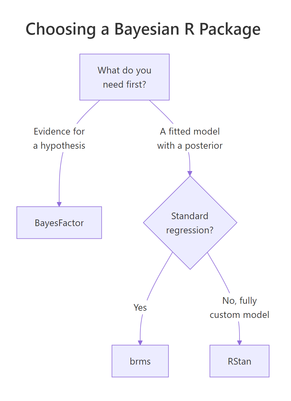
Figure 1: The one-question decision. Evidence for a hypothesis goes to BayesFactor, a standard regression goes to brms, and a fully custom model goes to RStan.
The same logic drives the recommend_package() function from the start of this guide. Point it at a real question and it returns the tool:
A conversion comparison is a yes/no question about a difference, so the function points you at BayesFactor. Change the question to "estimate the effect of price on demand across regions" and you are fitting a model, which sends you to brms. Only a model that no formula can express sends you to RStan.
Try it: A team needs a standard logistic regression with partial pooling by region. It is a fitting job, not a hypothesis test, and the formula interface handles it. Which package should they use?
Click to reveal solution
Explanation: Partial pooling is a multilevel model, and brms writes multilevel models from a formula like y ~ x + (1 | region). No Bayes factor and no custom code means the default answer, brms.
Practice Exercises
These combine the ideas above. Work them in your own R session; each is solvable with what this guide covered.
Exercise 1: Route three projects to the right package
You are advising three teams. Build a data.frame with a needs_bf and a custom flag for each project, then use mapply() with recommend_package() to fill a package column. The projects: (1) predict house prices with a multilevel model, (2) decide if treatment A beats treatment B, (3) build an ecological model with a custom likelihood.
Click to reveal solution
Explanation: The multilevel prediction is a fitting job with no special structure, so brms. The A/B decision is a hypothesis test, so BayesFactor. The custom likelihood cannot be written as a formula, so RStan. One function routed all three.
Exercise 2: Test a hypothesis and choose the package
A colleague flipped a coin 100 times and got 60 heads. They want to know whether that is real evidence against a fair coin. Use proportionBF() from BayesFactor to compute the Bayes factor against p = 0.5, then decide which package this question belonged to and whether the evidence is strong.
# Use proportionBF(y = 60, N = 100, p = 0.5) from BayesFactor.
# Then decide: is a Bayes factor near 1.6 strong evidence?
# Write your code here:
Click to reveal solution
set.seed(7)
# 60 heads in 100 flips. Evidence against a fair coin (p = 0.5)?
proportionBF(y = 60, N = 100, p = 0.5)
#> Bayes factor analysis
#> --------------
#> [1] Alt., p0=0.5, r=0.5 : 1.594878 ±0%
#>
#> Against denominator:
#>   Null, p = 0.5
#> ---
#> Bayes factor type: BFproportion, logistic
Explanation: This is a yes/no question about a hypothesis, so BayesFactor is the right package. The Bayes factor is about 1.6, barely above 1, so 60 heads in 100 flips is weak evidence at best. A single number, honestly reported, keeps you from over-claiming.
Frequently Asked Questions
Is brms just a wrapper for Stan?
Yes, and that is the point. brms translates your formula into a Stan program (the one you saw from make_stancode()), compiles it, and runs it through Stan's sampler. You get Stan's speed and reliability without writing Stan code. RStan is the lower-level interface to the same engine.
Can brms compute Bayes factors too?
It can, through bayes_factor() on two fitted brms models, but it needs careful priors and heavy sampling to do it well. BayesFactor is purpose-built for Bayes factors on common designs (t-tests, ANOVA, regression, correlation, proportions) and is far simpler for those cases. Use the right tool for the question.
Is rstanarm the same as brms?
They are close cousins. Both let you fit Bayesian regression with R formula syntax on top of Stan. rstanarm ships precompiled models, so it skips the per-model compile step, but it covers a smaller set of models. brms compiles each model yet supports a much wider range, which is why it is the more common recommendation for flexible work.
Do I need to know Stan to use brms?
No. The whole appeal of brms is that you never open a Stan file. You should understand priors and posteriors, which the parent guide on Bayesian statistics covers, but the Stan code stays under the hood unless you choose to inspect it.
Why is BayesFactor sometimes discouraged for general use?
BayesFactor is excellent for the standard tests it implements, but it does not give you a full posterior for arbitrary models, and it can be slow or unavailable for large or unusual designs. For general model fitting with uncertainty estimates, brms is the broader tool. For clean hypothesis tests, BayesFactor is hard to beat.
Summary
| Package | Best for | Gives you back | You write | Trade-off |
|---|---|---|---|---|
| brms | Applied regression, multilevel and non-Gaussian models | A full posterior | One formula | Compiles each model |
| RStan | Fully custom models no formula can express | A full posterior | The Stan program yourself | Most code and setup |
| BayesFactor | Hypothesis tests on standard designs | A single Bayes factor | One test call | No posterior for custom models |
The one-line takeaway: default to brms, drop to RStan only when a formula cannot express your model, and switch to BayesFactor when the question is which hypothesis the data support rather than what the fitted model looks like.
References
- Bürkner, P. C. brms: An R Package for Bayesian Multilevel Models Using Stan. Journal of Statistical Software (2017). Link
- brms package on CRAN. Link
- RStan: the R interface to Stan. Link
- BayesFactor package on CRAN. Link
- Morey, R. D. BayesFactor package documentation. Link
- rstanarm: Bayesian applied regression modeling via Stan. Link
- bayestestR: describe posteriors from brms, rstanarm, and BayesFactor. Link
Continue Learning
- Bayesian Statistics in R: the prior, likelihood, and posterior foundations this guide builds on.
- brms in R: a deeper walkthrough of fitting and interpreting brms models.
- Bayes Factors in R: how to compute and read Bayes factors with the BayesFactor package.