Bayesian Survival Analysis in R: rstanarm Package
Bayesian survival analysis models the time until an event, like death or a machine failure, while properly handling patients who never had the event during the study. Instead of a single number for each effect, it returns a full posterior distribution, so you can make direct probability statements. In R, the rstanarm package fits these models behind a familiar formula interface, with Stan doing the sampling for you.
This is a companion to Bayesian Logistic Regression in R. There you modeled a yes/no outcome. Here the outcome is a time, and the twist is that some of those times are only partially known. We will build the idea from the ground up: what survival data is, how to summarize it, and then how to fit and read a Bayesian model with rstanarm. Every result below comes from real R output.
What does survival analysis actually measure?
Survival analysis studies how long it takes for something to happen. The "something" is an event: a patient dies, a customer cancels, a part breaks. The measurement is the time from a starting point until that event. The catch that makes survival its own field is that for many subjects the event has not happened yet when the study ends. You know they lasted at least so long, but not their final time. That partial knowledge is called censoring, and throwing those subjects away would bias your answer.
Let's look at a real dataset. The survival package ships with veteran, a lung-cancer trial of 137 patients. The key columns are time (days of follow-up), status (1 if the patient died, 0 if still alive at the study's end), and karno, the Karnofsky performance score that rates how well a patient can carry out daily activities.
Each row is one patient. A status of 1 means we saw the death and know the exact survival time. A status of 0 means the patient was censored. R has a dedicated type for this pairing: the Surv() object. It bundles the time and the event flag together, and it prints a + next to censored times to remind you the true survival time is longer than what you see.
The tenth patient shows as 100+. They were followed for 100 days and were still alive, so their real survival time is unknown but at least 100 days. A Bayesian model, like every good survival method, uses that "at least" information instead of discarding it.
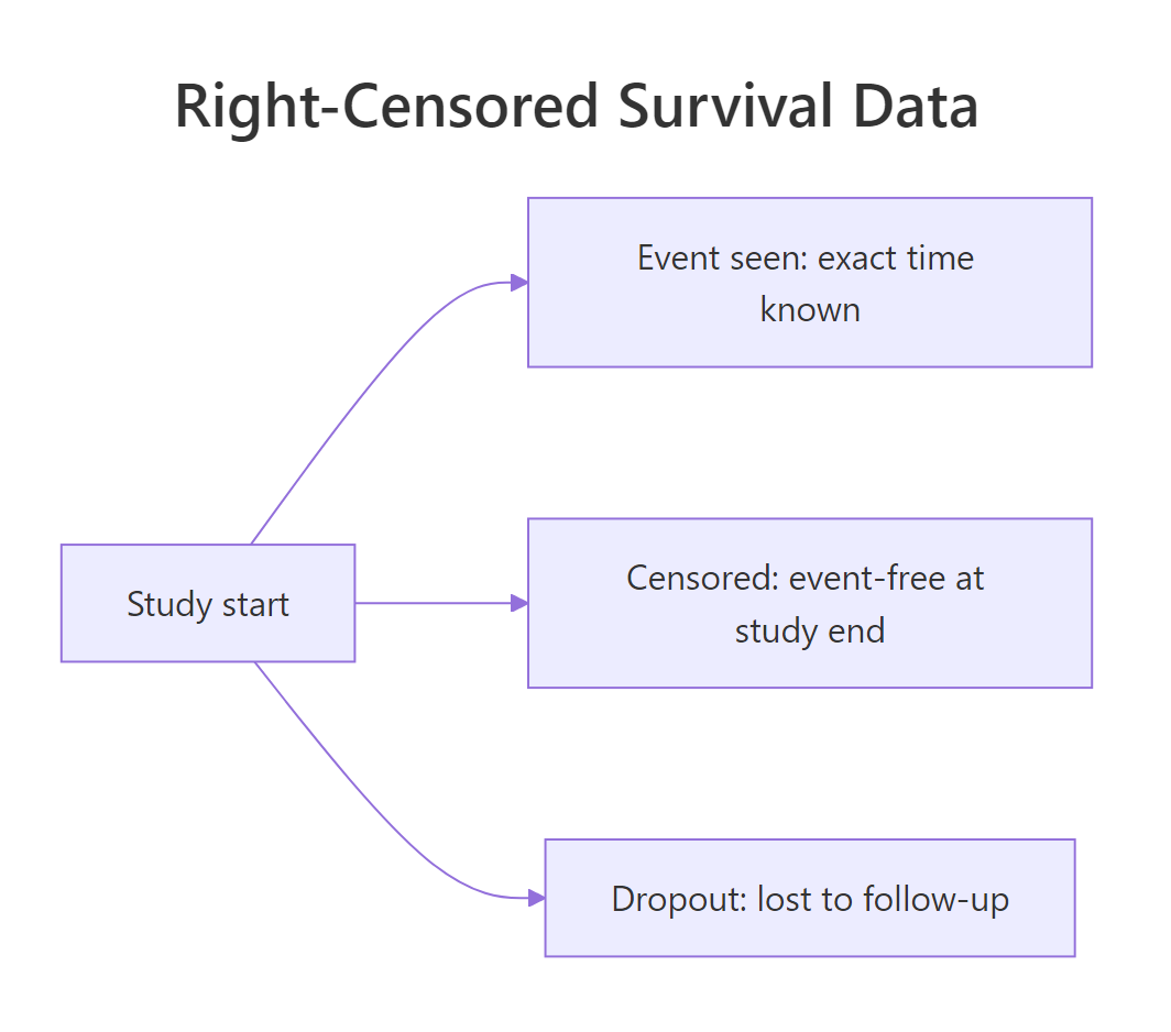
Figure 1: Three ways a patient's follow-up can end. Only exact-event times are fully observed; censored patients still contribute the information that they survived up to their last recorded day.
Try it: Count how many of the 137 patients were censored (their status equals 0).
Click to reveal solution
Explanation: status == 0 is a logical vector that is TRUE for censored patients, and sum() counts the TRUE values. Nine of the 137 patients were still alive when the study ended.
How do you estimate survival without any model?
Before fitting anything, you want a picture of survival over time. The standard tool is the Kaplan-Meier estimator. It walks through the ordered event times and, at each death, drops the estimated survival probability by the fraction of still-at-risk patients who died. Censored patients simply leave the at-risk pool without causing a drop. The result is a step curve: the estimated probability of surviving past any given day.
The most useful single number it produces is the median survival time, the day by which half the group has had the event. Let's relabel the two treatment arms first so every table reads clearly, then compute the overall curve.
Across all 137 patients, the median survival is 80 days, with a 95% confidence interval from 52 to 105 days. Now split the estimate by treatment arm to see whether the experimental therapy helped.
The standard arm has a median of 103 days versus 52.5 for the test arm. On this raw view the experimental treatment looks worse, though the confidence intervals overlap heavily. A curve makes the gap easier to read than a table.
Each step down marks a day when at least one patient died. The two curves cross and stay close, which is a hint that the treatment effect, if any, is small. Kaplan-Meier is a great summary, but it cannot adjust for other variables like the Karnofsky score. For that you need a model.
Try it: Read the median survival for just the standard arm from the km_trt object above.
Click to reveal solution
Explanation: summary(km_trt)$table returns one row per arm; the median column holds each arm's median survival time. The standard arm's median is 103 days.
How does a Cox model turn covariates into hazard ratios?
The most common survival model is Cox proportional hazards. It models the hazard, the instantaneous risk of the event at each moment for a patient who has survived that long. The Cox model says each covariate multiplies that hazard by a fixed factor, the hazard ratio. A hazard ratio above 1 means higher risk (shorter survival); below 1 means lower risk (longer survival). You will meet the same hazard ratio in the Bayesian model, so it is worth pinning down here with the familiar frequentist fit.
The exp(coef) column is the hazard ratio. For karno it is 0.967: each one-point rise in the Karnofsky score multiplies the hazard by 0.967, a roughly 3% lower risk of death per point, and its tiny p-value says this is a strong signal. For trttest the hazard ratio is 1.19, meaning the test arm carries about 19% higher risk, but the p-value of 0.33 says the data are consistent with no difference at all. These point estimates are exactly what a Bayesian fit will replace with full distributions.
Try it: Refit the Cox model with age added as a third covariate and read its hazard ratio.
Click to reveal solution
Explanation: Age has a hazard ratio of 0.996, essentially 1, so it barely shifts risk once treatment and Karnofsky score are accounted for. Karnofsky remains the dominant predictor.
How do you fit a Bayesian survival model with rstanarm?
Here is the honest lay of the land. The current CRAN release of rstanarm does not ship a dedicated stan_surv() function; that lives on a development branch. What you can do on stock CRAN is exploit a classic equivalence: the simplest survival model, the exponential model, is identical to a Poisson regression on the event indicator with the log of follow-up time as an offset. That means stan_glm() fits it directly.
The reasoning is short. An exponential model assumes a constant hazard $h$ for each patient. The chance of the event during a follow-up of length $t$ then behaves like a Poisson count with mean $h \cdot t$, where the observed count is the event indicator (0 or 1). Taking logs:
$$\log(h_i \cdot t_i) = \log(t_i) + \beta_0 + \beta_1 x_{i1} + \dots$$
The $\log(t_i)$ term is a known quantity per patient, an offset, and the rest is an ordinary log-linear model. So a Poisson regression of status on the covariates, offset by log(time), is the exponential survival model.
offset = log(time), and the coefficients are log hazard ratios, exactly the quantities a Cox model reports.One practical caveat before you run the fit.
seed = 2024.library(rstanarm)
# Poisson regression of the event indicator with a log-time offset
# IS the exponential survival model. seed makes the draws reproducible.
fit_exp <- stan_glm(
status ~ trt + karno + offset(log(time)),
data = veteran,
family = poisson(link = "log"),
chains = 4, iter = 2000, seed = 2024, refresh = 0
)
print(fit_exp, digits = 3)
#> stan_glm
#> family: poisson [log]
#> formula: status ~ trt + karno + offset(log(time))
#> observations: 137
#> predictors: 3
#> ------
#> Median MAD_SD
#> (Intercept) -2.713 0.283
#> trttest 0.131 0.181
#> karno -0.035 0.005The output is a posterior summary, not a single fit. Each Median is the middle of that coefficient's posterior distribution, and MAD_SD is a robust posterior standard deviation. The karno coefficient sits at -0.035 with a small spread, while trttest at 0.131 has a spread (0.181) wider than the estimate itself, an early sign its effect is uncertain. These are log hazard ratios; the next section turns them into hazard ratios you can read.
Try it locally: What is the posterior probability that the test arm has a higher hazard than the standard arm? That is the probability its coefficient is above 0.
# Pull the posterior draws with as.matrix(fit_exp), then ask what fraction
# of the trttest column is greater than 0.
# mean(as.matrix(fit_exp)[, "trttest"] > 0)
Click to reveal solution
mean(as.matrix(fit_exp)[, "trttest"] > 0)
#> [1] 0.7645
Explanation: About 76% of the posterior mass for the treatment coefficient is above 0, so there is roughly a 76% chance the test arm is worse and a 24% chance it is actually better. That is a far more honest summary than a yes/no verdict from a p-value.
How do you read hazard ratios from the posterior?
A log hazard ratio is awkward to explain. Exponentiate it and you get the hazard ratio itself, on the same scale the Cox model used. Because the posterior is just a big pile of draws, you can exponentiate every draw and read off a median and an interval directly. The posterior_interval() function gives a credible interval; with prob = 0.90 it returns the 5th and 95th percentiles of the posterior.
# exp() of each coefficient (and its interval) is a hazard ratio.
hr <- exp(cbind(HR = coef(fit_exp), posterior_interval(fit_exp, prob = 0.90)))
round(hr[c("trttest", "karno"), ], 3)
#>            HR    5%   95%
#> trttest 1.140 0.844 1.507
#> karno   0.965 0.958 0.973
The test arm's hazard ratio is 1.14 with a 90% credible interval from 0.84 to 1.51. Because that interval comfortably includes 1, the data do not pin down whether the treatment helps or hurts. The Karnofsky hazard ratio is 0.965 with a tight interval from 0.958 to 0.973, entirely below 1: healthier patients reliably live longer. Now compare these to the Cox estimates from earlier.
cox_hr   <- exp(coef(cox)[c("trttest", "karno")])
bayes_hr <- exp(coef(fit_exp)[c("trttest", "karno")])
round(data.frame(cox_HR = cox_hr, bayes_HR = bayes_hr), 3)
#>         cox_HR bayes_HR
#> trttest  1.194    1.140
#> karno    0.967    0.965
The two approaches land in almost the same place. That agreement is reassuring: the Bayesian machinery is not inventing a different answer, it is giving the same central estimates plus a genuine probability distribution around them. The difference is in interpretation.
exp(as.matrix(fit)[, "trttest"]) gives you thousands of plausible hazard ratios you can histogram, average, or threshold, no extra modeling needed.Try it locally: Report the 90% credible interval for the karno hazard ratio using the posterior draws directly.
# Take the karno column of as.matrix(fit_exp), exp() it, and read the
# 5th and 95th percentiles with quantile().
# round(exp(quantile(as.matrix(fit_exp)[, "karno"], c(0.05, 0.95))), 3)
Click to reveal solution
round(exp(quantile(as.matrix(fit_exp)[, "karno"], c(0.05, 0.95))), 3)
#>    5%   95%
#> 0.958 0.973
Explanation: The interval matches the one from posterior_interval(), because both read the same percentiles off the same posterior draws. Every point in it is below 1, so a higher Karnofsky score is very likely protective.
How do you get a survival probability with full uncertainty?
Hazard ratios answer "who is at higher risk", but patients and stakeholders usually want a probability: what are the chances of surviving past six months? For the exponential model the survival function has a clean form. With a constant hazard $h$, the probability of surviving past time $t$ is:
$$S(t) = e^{-h t}$$
In a Bayesian workflow $h$ is not one number, it is a whole posterior distribution. Push every posterior draw through that formula and you get a full distribution for the survival probability, complete with a credible interval. Let's do it for a specific patient: someone in the test arm with a Karnofsky score of 60, at 90 days.
draws   <- as.matrix(fit_exp)     # one row per posterior draw
# Linear predictor for a test-arm patient with Karnofsky score 60:
log_haz <- draws[, "(Intercept)"] + draws[, "trttest"] * 1 + draws[, "karno"] * 60
haz     <- exp(log_haz)           # this patient's constant hazard, per draw
S90     <- exp(-haz * 90)         # probability of surviving past 90 days

round(c(mean = mean(S90), median = median(S90),
        lo = quantile(S90, 0.05), hi = quantile(S90, 0.95)), 3)
#>    mean median  lo.5% hi.95%
#>   0.438  0.437  0.367  0.512
The model's best guess is a 44% chance this patient survives past 90 days, and it is 90% sure the true probability sits between 37% and 51%. That interval is the honest expression of what the data support. You can also ask direct probability questions of the same draws.
# What is the chance this patient does NOT survive 90 days?
mean(S90 < 0.5)
#> [1] 0.916
There is a 92% posterior probability that this patient's true 90-day survival is below 50%. This kind of plain-language probability is the payoff of going Bayesian: the uncertainty is baked into every answer instead of bolted on afterward.
Try it locally: Compute the posterior mean survival probability at 180 days for the same patient profile.
# Reuse the haz vector, but push it through exp(-haz * 180) this time.
# round(mean(exp(-haz * 180)), 3)
Click to reveal solution
round(mean(exp(-haz * 180)), 3)
#> [1] 0.194
Explanation: Doubling the horizon to 180 days drops the mean survival probability to about 19%. Under a constant hazard, survival probability decays geometrically, so longer horizons fall off quickly.
How do priors shape the answer?
Every Bayesian model needs priors, the starting beliefs about each coefficient before seeing data. rstanarm picks weakly-informative defaults and rescales them to your data automatically, so you rarely have to think about them, but you should know what they are. The prior_summary() function shows both what you asked for and the adjusted version rstanarm actually used.
prior_summary(fit_exp)
#> Priors for model 'fit_exp'
#> ------
#> Intercept (after predictors centered)
#>  ~ normal(location = 0, scale = 2.5)
#>
#> Coefficients
#>   Specified prior:
#>     ~ normal(location = [0,0], scale = [2.5,2.5])
#>   Adjusted prior:
#>     ~ normal(location = [0,0], scale = [4.98,0.12])
#> ------
#> See help('prior_summary.stanreg') for more details
The defaults are normal distributions centered at 0, meaning "no effect" is the starting assumption. The adjusted scales (4.98 and 0.12) are rescaled to the spread of each predictor, so karno, which ranges into the dozens, gets a tighter coefficient prior than the binary treatment indicator. With 137 patients the data far outweigh these weak priors, so the defaults barely affect the result here. To see a prior actually shift an estimate, tighten it and refit.
fit_prior <- stan_glm(
  status ~ trt + karno + offset(log(time)), data = veteran,
  family = poisson(link = "log"),
  prior = normal(0, 0.5), prior_intercept = normal(-5, 2),
  chains = 4, iter = 2000, seed = 2024, refresh = 0
)
round(cbind(default = coef(fit_exp), tighter = coef(fit_prior)), 3)
#>             default tighter
#> (Intercept)  -2.713  -2.713
#> trttest       0.131   0.109
#> karno        -0.035  -0.035
The tighter prior pulls the uncertain trttest coefficient from 0.131 toward 0 (down to 0.109), because a prior centered at 0 exerts more pull when the data are weak. The well-identified karno coefficient does not budge. That is exactly how priors should behave: they stabilize the estimates the data cannot pin down, and have almost no effect where the data are already strong.
Try it locally: What is the posterior probability that a higher Karnofsky score lowers the hazard (its coefficient is below 0)?
# Ask what fraction of the karno posterior draws are below 0.
# mean(as.matrix(fit_exp)[, "karno"] < 0)
Click to reveal solution
mean(as.matrix(fit_exp)[, "karno"] < 0)
#> [1] 1
Explanation: Every posterior draw for the karno coefficient is below 0, so the model is essentially certain that a higher Karnofsky score is protective. That certainty comes from the strong signal in the data, not from the prior.
What if the hazard changes over time?
The exponential model assumes each patient's hazard is constant for all time, which is often too rigid: risk can rise or fall as a disease progresses. The piecewise-exponential model relaxes this. It chops follow-up into intervals and lets the baseline hazard take a different constant value in each one, while covariate effects stay proportional. The Poisson trick still works; you just split each patient into one row per interval they pass through and add the interval as a factor. The survSplit() function does the splitting.
Every patient contributes a record to interval 1, but only the 73 who survived past 60 days reach interval 2, and so on. Each record carries an exposure, the time actually spent in that band, which becomes the new offset. Now fit the model with an interval factor for the flexible baseline.
fit_pw <- stan_glm(
  status ~ factor(interval) + trt + karno + offset(log(exposure)),
  data = vet_split, family = poisson(link = "log"),
  chains = 4, iter = 2000, seed = 2024, refresh = 0
)
round(coef(fit_pw), 3)
#>       (Intercept) factor(interval)2 factor(interval)3 factor(interval)4           trttest
#>            -2.734            -0.125            -0.084            -0.378             0.137
#>             karno
#>            -0.033
The factor(interval) terms are the baseline-hazard adjustments per band. They are all small and negative here (the largest, -0.378 for interval 4), meaning the baseline hazard is fairly flat and drifts slightly downward over time in this trial. Crucially, the trttest and karno coefficients (0.137 and -0.033) barely move from the exponential fit. For this dataset the simpler constant-hazard model was already adequate, and now you have checked that rather than assumed it.
Try it: How many deaths happened in the first interval (the first 60 days)?
Click to reveal solution
Explanation: 63 of the 128 deaths occur in the first 60 days, nearly half. That heavy early mortality is why the median survival was only 80 days.
Frequently asked questions
Is this the same as the stan_surv() function I have seen in tutorials? Not quite. stan_surv() is a dedicated survival interface that lives on the rstanarm development branch and offers Weibull, Gompertz, and spline hazards. The CRAN release you install with install.packages("rstanarm") does not include it. The Poisson-offset approach here uses only CRAN rstanarm and gives you the exact exponential and piecewise-exponential models.
Can rstanarm fit a Bayesian Cox model directly? Not on CRAN. The Cox model leaves the baseline hazard unspecified, which needs the development stan_surv() or the brms package. The piecewise-exponential model above is the practical stand-in: make the intervals fine enough and it approximates the flexible Cox baseline while staying fully on CRAN.
How many iterations and chains should I use? The defaults, 4 chains of 2000 iterations each, are a sensible start. Increase the iterations if the effective sample size is low or the estimates look unstable across runs. Always check convergence before trusting the numbers.
How do I know the sampler converged? Look at two diagnostics from summary(fit_exp): Rhat should be at or very near 1.00 for every parameter, and n_eff (the effective sample size) should be in the hundreds or more. Values of Rhat above about 1.01 mean the chains disagree and you should sample longer.
Why an exponential model and not Weibull? The exponential model assumes a constant hazard, which is the simplest honest starting point and maps cleanly onto stan_glm(). The Weibull model lets the hazard rise or fall smoothly with time. For a Bayesian Weibull fit on CRAN, reach for brms; the piecewise-exponential model here is a flexible non-parametric alternative when you want to stay in rstanarm.
Practice Exercises
These build on the fitted objects above (fit_exp and its posterior draws). They run in R with rstanarm loaded, not in the in-page runner.
Exercise 1: Combine two probability statements
Using the posterior draws of fit_exp, estimate the probability that the test arm is worse than standard (its hazard ratio exceeds 1) and a higher Karnofsky score is protective (its coefficient is below 0), both at once. Save the result to p_both.
# Hint: pull as.matrix(fit_exp) once, then combine two conditions with &.

# Write your code below:
Click to reveal solution
post   <- as.matrix(fit_exp)
p_both <- mean(post[, "trttest"] > 0 & post[, "karno"] < 0)
round(p_both, 3)
#> [1] 0.764
Explanation: The joint condition is TRUE on 76% of the draws, which nearly equals the treatment-is-worse probability alone because the Karnofsky-is-protective condition is almost always TRUE. Combining conditions on the raw draws is how Bayesian analysis answers compound questions.
Exercise 2: Compare two patients' survival
For a test-arm patient, compute the posterior mean probability of surviving past 180 days for a strong Karnofsky score of 90 versus a weak score of 40. Then report the probability that the strong patient's survival exceeds the weak patient's. Reuse the posterior draws.
# Hint: write the linear predictor as a function of the Karnofsky score k,
# then push each through exp(-exp(lp) * 180) and average.

# Write your code below:
Click to reveal solution
post <- as.matrix(fit_exp)
lp   <- function(k) post[, "(Intercept)"] + post[, "trttest"] + post[, "karno"] * k
S_strong <- exp(-exp(lp(90)) * 180)
S_weak   <- exp(-exp(lp(40)) * 180)
round(c(strong = mean(S_strong), weak = mean(S_weak),
        p_strong_better = mean(S_strong > S_weak)), 3)
#>          strong            weak p_strong_better
#>           0.561           0.039           1.000
Explanation: The strong-Karnofsky patient has a 56% mean chance of surviving 180 days versus 4% for the weak one, and the strong patient does better in every posterior draw (probability 1.00). The performance score dominates outcome in this trial.
Summary
Bayesian survival analysis handles censored time-to-event data and returns full posterior distributions instead of point estimates. On stock CRAN rstanarm, you fit these models by recognizing the exponential survival model as a Poisson regression with a log-time offset, then reading hazard ratios and survival probabilities straight off the posterior draws.
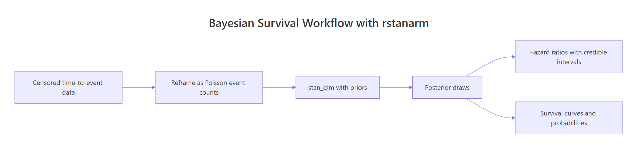
Figure 2: The rstanarm survival workflow. Reframe censored data as Poisson event counts, fit with priors using stan_glm, then read hazard ratios and survival curves from the posterior draws.
| Concept | What to remember |
|---|---|
| Censoring | A censored row means "survived at least this long"; never drop it. |
| Kaplan-Meier | Model-free survival curve and median; cannot adjust for covariates. |
| The Poisson trick | Exponential survival = Poisson regression of the event flag with offset = log(time). |
| Hazard ratio | exp(coefficient); above 1 is higher risk, below 1 is lower risk. |
| Credible interval | A genuine probability statement about the parameter, unlike a confidence interval. |
| Survival probability | Push posterior draws through S(t) = exp(-h t) for a full distribution. |
| Piecewise-exponential | Split time with survSplit() to let the baseline hazard vary. |
References
- Goodrich, B., Gabry, J., Ali, I., & Brilleman, S. rstanarm: Bayesian Applied Regression Modeling via Stan. CRAN package page. Link
- Brilleman, S. L., Elci, E. M., Novik, J. B., & Wolfe, R. Bayesian Survival Analysis Using the rstanarm R Package. arXiv:2002.09633 (2020). Link
- Therneau, T. M. survival: Survival Analysis. CRAN package page. Link
- Stan Development Team. rstanarm documentation and vignettes. Link
- Gabry, J., & Goodrich, B. Prior Distributions for rstanarm Models. Link
- Bürkner, P.-C. brms: Bayesian Regression Models using Stan. CRAN package page. Link
Continue Learning
- Bayesian Logistic Regression in R: the binary-outcome companion that introduces the same posterior-and-prior machinery on an easier model.
- Bayesian Linear Regression in R: start here if you want the gentlest introduction to reading a Bayesian posterior.
- RStan vs brms vs BayesFactor in R: decide which Bayesian package fits your problem before you commit.