Prior Sensitivity Analysis in R: Does the Prior Matter?
Prior sensitivity analysis means refitting a Bayesian model under a range of reasonable priors and checking whether your conclusion changes. If the answer stays the same, the result is robust. If it flips, the prior, not the data, is driving your answer. This post shows you how to run that check from scratch, work out exactly when the prior matters, and connect it to the tools you use for real models.
What is prior sensitivity analysis, and why should you care?
Imagine you run a small test of a new checkout button and see 8 conversions out of 20 visitors. You hand that result to three colleagues and ask each for their best estimate of the true conversion rate. One is cautious and expected a low rate. One is hopeful and expected a high rate. One has no opinion at all. In a Bayesian analysis, each of those starting opinions is a prior, and each colleague will hand you back a slightly different answer from the same 8-out-of-20 data.
Prior sensitivity analysis is the discipline of measuring that disagreement on purpose. A Bayesian posterior is a blend of two ingredients: the prior (what you believed before the data) and the likelihood (what the data says). When the data is plentiful, the blend is almost pure data and everyone lands in the same place. When the data is thin, the prior gets a real vote, and reasonable people with different priors can reach different conclusions.
Let us make the three colleagues concrete. We will describe each prior as a Beta distribution, which is the natural way to express a belief about a rate between 0 and 1. A Beta(a, b) prior has mean a / (a + b), so Beta(2, 8) leans low (mean 0.2) and Beta(8, 2) leans high (mean 0.8). The convenient part is that for count data like "8 successes out of 20," the posterior is also a Beta, with parameters Beta(a + successes, b + failures). This tidy pairing, where the posterior lands in the same Beta family as the prior, is called conjugacy. No simulation is needed; the answer is a formula you can evaluate directly.
Here is what that code did. We stored each colleague's prior as a pair of numbers (a, b), then applied the posterior formula Beta(a + k, b + n - k) and read off its mean (a + k) / (a + b + n). The unname() call just strips a stray label so the output stays tidy.
Now read the three numbers. From identical data, the cautious skeptic's best estimate is 0.333, the no-opinion analyst lands at 0.409, and the optimist reaches 0.533. That is a spread of two-tenths in the estimated conversion rate, produced entirely by the choice of prior. Whether that spread is a problem or a footnote is exactly the question prior sensitivity analysis answers.
Try it: Add a fourth, much stronger skeptic to the picture. A Beta(20, 80) prior also has mean 0.2, but it is far more confident. Compute its posterior mean and see how much harder it pulls.
Click to reveal solution
Explanation: The stronger Beta(20, 80) prior pulls the posterior mean all the way down to 0.233, much lower than the milder skeptic's 0.333. A more confident prior gets a bigger vote, so it bends the answer harder. The next section turns that "vote" into an exact number.
Why does changing the prior change your answer?
The reason the prior moves the answer is not mysterious, and you do not have to take it on faith. For this Beta-Binomial setup, the posterior mean is exactly a weighted average of the prior's mean and the data's own rate. You can write down the weights.
Let \(a + b\) be the prior's strength: it behaves like a number of imaginary trials the prior is "worth." A Beta(2, 8) prior is worth 10 imaginary trials; a Beta(20, 80) prior is worth 100. The data brings \(n\) real trials. The posterior mean splits its vote between the two in proportion to those counts.
$$\text{posterior mean} = w \times (\text{prior mean}) + (1 - w) \times (\text{data mean})$$
$$w = \frac{a + b}{a + b + n}$$
Where \(w\) is the share of the answer that comes from the prior, \(a + b\) is the prior's strength in imaginary trials, and \(n\) is the number of real trials in your data. The rest of the vote, \(1 - w\), goes to the data. This one fraction is the whole story of "does the prior matter." Let us compute it for our three colleagues.
Walk across one row. The skeptic's prior is worth 10 imaginary trials against 20 real ones, so its weight is 10 / (10 + 20) = 0.333. The posterior mean is then 0.333 * 0.2 + 0.667 * 0.4 = 0.333, exactly the number in the table. The vague prior is worth only 2 trials, so it gets a 9% vote and barely nudges the answer off the raw data rate of 0.4.
That is why the optimist and the skeptic disagreed in section 1: each held a prior worth 10 trials, so each grabbed a third of a 20-trial answer and pulled it toward their own belief. The vague analyst held almost no weight and landed on the data.
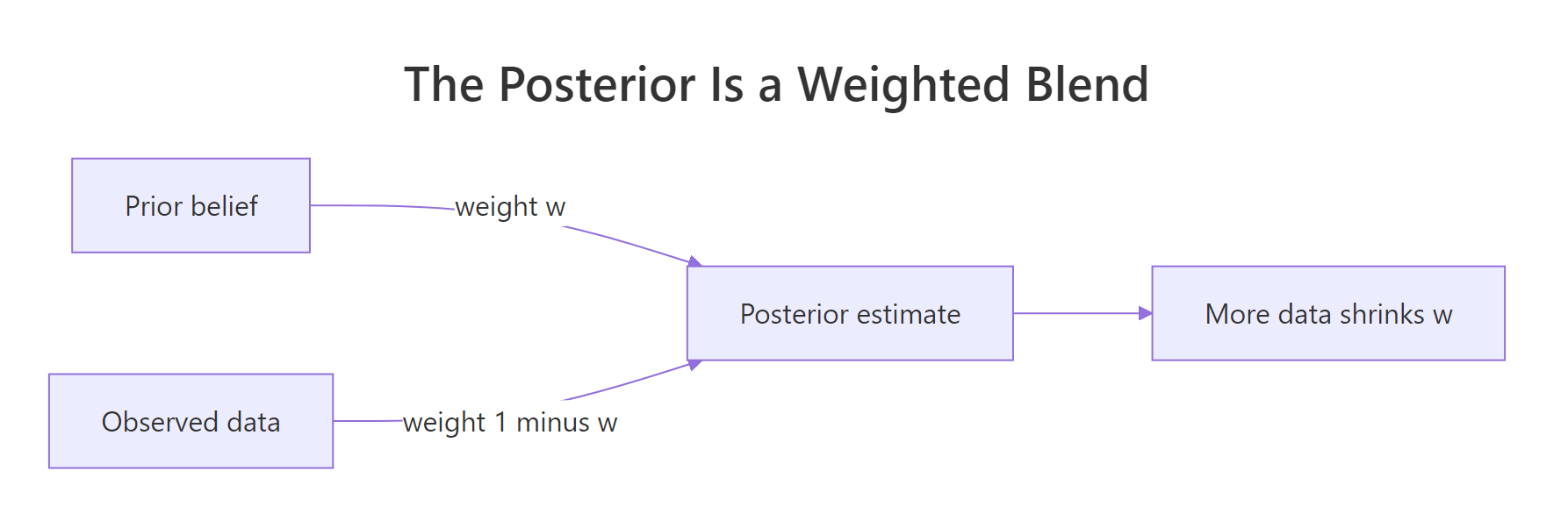
Figure 1: The posterior estimate is a weighted blend of the prior and the data; more data shrinks the prior's weight w toward zero.
The same logic holds for continuous quantities like a mean, where the weights are precisions (one divided by the variance) instead of trial counts. A tight prior has high precision and a big weight; a diffuse prior has low precision and a small one. The vocabulary changes, but the tug-of-war is identical.
Try it: The skeptic prior is worth 10 trials. How many real visitors \(n\) would you need before its weight drops below 10%? Solve 10 / (10 + n) < 0.10.
Click to reveal solution
Explanation: Past about 90 visitors, the skeptic prior holds less than a tenth of the vote, so its influence on the answer is minor. Below that, it is a genuine player. Knowing this number for your own prior tells you at a glance whether your dataset is large enough to ignore the argument.
How do you actually run a prior sensitivity analysis?
You now understand why priors matter. Running a sensitivity analysis turns that understanding into a short, repeatable procedure you can bolt onto the end of any Bayesian analysis. There are four steps.
- State the decision your analysis feeds. Not "estimate the rate," but the actual call you will make, such as "ship the button only if we are at least 90% sure the true rate beats the 0.35 break-even point."
- Pick a panel of priors that spans what reasonable people believe: a vague prior, a mild default, a skeptic, an enthusiast, and any prior drawn from earlier studies.
- Refit under each prior and record both the posterior summary and the decision quantity.
- Read the table. If the decision is the same under every prior, it is robust. If it flips, it is prior-sensitive, and you have a story to tell about how much your assumptions contributed.
First we need a small helper that reports what we care about for one prior: the posterior mean, a 95% credible interval (the range that holds 95% of the posterior), and the probability the rate clears our threshold.
The helper uses qbeta() to read percentiles off the posterior Beta and pbeta(..., lower.tail = FALSE) to get the probability the rate exceeds the threshold. For the vague prior, there is a 70.6% chance the true rate beats 0.35: promising, but short of a confident "ship it." Now run the whole panel through it.
Read the p_above column against our decision rule, "ship only if the probability of clearing 0.35 is at least 0.90." Only the optimist clears the bar, at 0.979. Everyone else lands between 0.003 and 0.741. The recommendation is not "ship" or "wait"; it depends entirely on whose prior you trust. With 20 visitors, this decision is prior-sensitive, and reporting only the optimist's answer would be misleading.

Figure 2: The prior sensitivity analysis loop. Refit the same model under a panel of priors, then read whether the decision holds or flips.
Now collect ten times as much data, keeping the same 40% observed rate, and rerun the identical panel.
Look at the post_mean column now. The four reasonable priors cluster between 0.390 and 0.419, a spread of three-hundredths, down from the two-tenths gulf at 20 visitors. The data has bought most of the robustness. The one holdout is strong_skeptic, still at 0.333, because a prior worth 100 imaginary trials still holds a third of the vote even against 200 real ones.
Beta(20, 80) prior still bends your 200-trial result, the fix is not more data; it is justifying, or dropping, a prior that asserts the equivalent of 100 prior observations you may not actually have.Try it: Rerun the 20-visitor sweep with an easier threshold of 0.30 instead of 0.35, and compare the p_above column to the table above. Which way does every prior move, and by how much does that depend on the prior?
Click to reveal solution
Explanation: Every prior grows more confident when the bar drops from 0.35 to 0.30, because clearing an easier target is more probable. But the size of the jump depends on the prior: the optimist barely changes (already near 1), while the milder skeptic climbs from 0.408 to 0.636. The strong_skeptic stays far below the bar at 0.048. Moving the threshold and moving the prior are two different levers, and a good analysis reports sensitivity to both.
What if your model has no conjugate shortcut?
The Beta-Binomial trick worked because the posterior had a clean formula. Most real priors and models do not. The moment you want a prior that is not a Beta, or a model without a tidy conjugate partner, you need a method that works for any prior. The simplest such method is a grid: chop the parameter range into many points, and compute the posterior weight at each one by hand.
The recipe is three lines. At every candidate rate on the grid, multiply the prior density by the likelihood of your data, then divide by the total so the weights sum to one. Swap in a different prior and you get a different posterior from the same data, with no formula required.
The grid posterior mean for the skeptic prior is 0.333, matching the exact conjugate answer to three decimals. That agreement is your proof that the grid method is trustworthy: when a formula exists, the grid reproduces it. Now use it for a prior that has no conjugate form at all, such as a "two camps" mixture that puts half its belief on the skeptic's bump and half on the optimist's.
The mixed prior lands at 0.364, between the skeptic's 0.333 and the raw data's 0.4, which is exactly where a blend of a low bump and a high bump should sit once the data leans low. There is no closed form for this posterior, yet the grid handled it without complaint. Plotting the full posteriors side by side makes the effect of the prior visible at a glance.
The plot shows four posteriors built from the same 8-out-of-20 data. The skeptic's curve sits to the left of the dashed data line, the optimist's to the right, and the vague and mixture curves straddle it. Seeing the curves shift is the most persuasive way to communicate prior sensitivity to a non-technical audience, because the disagreement is right there in the picture.
Try it: Build a symmetric, moderately informative prior with Beta(5, 5) (mean 0.5, worth 10 trials) and find its posterior mean on the grid.
Click to reveal solution
Explanation: The symmetric Beta(5, 5) prior pulls the posterior toward its own mean of 0.5, landing at 0.433, above the data rate of 0.4. Even a prior that looks "neutral" is informative: a mean of 0.5 is a genuine claim, and worth 10 trials it takes a real bite out of a 20-trial dataset.
How do you check prior sensitivity in a real regression?
Conjugate math and grids are perfect for teaching, but your real models will be regressions, hierarchical models, and generalized linear models fit with a sampler. You cannot write their posteriors by hand. The good news is that the workflow does not change: pick a panel of priors, refit the model under each, and compare. Packages like rstanarm and brms make the refit a one-line change, because you can fit once and then update only the prior.
The block below fits a simple linear regression twice on the same simulated data. The first fit uses a sensible weakly informative prior on the slope; the second changes only that prior to a tight, skeptical normal(0, 0.2) and refits. This code uses a sampler that runs outside the browser, so run it in your own R session with rstanarm installed.
suppressPackageStartupMessages(library(rstanarm))

set.seed(2026)
n_obs <- 30
sim <- data.frame(x = rnorm(n_obs))
sim$y <- 1 + 0.6 * sim$x + rnorm(n_obs)   # true slope = 0.6

# Weakly informative prior on the slope
fit_weak <- stan_glm(y ~ x, data = sim,
                     prior = normal(0, 5),
                     chains = 2, iter = 1000, seed = 123, refresh = 0)

# Refit with ONLY the slope prior changed to a tight, skeptical normal(0, 0.2)
fit_tight <- update(fit_weak, prior = normal(0, 0.2))

comparison <- rbind(
  weak_prior  = posterior_interval(fit_weak,  prob = 0.9, pars = "x")["x", ],
  tight_prior = posterior_interval(fit_tight, prob = 0.9, pars = "x")["x", ]
)
round(comparison, 2)
#>               5%  95%
#> weak_prior  0.36 0.79
#> tight_prior 0.19 0.58
The true slope was 0.6. Under the weakly informative prior, the 90% credible interval is [0.36, 0.79], comfortably around the truth. Swap in the tight skeptical prior and the same 30 observations produce [0.19, 0.58], shifted noticeably toward zero. The update() call is the whole trick: it reuses the fitted model and changes only the prior, so a full sweep over five priors is five short lines. The verdict reads exactly like the conjugate sweeps earlier, because it is the same idea applied to a model you cannot solve by hand.
There is also an automated shortcut worth knowing. Instead of refitting under a handful of hand-picked priors, power-scaling gently strengthens or weakens your existing prior and measures how much the posterior reacts, all from a single fit. The priorsense package by Kallioinen and colleagues implements this with an efficient importance-sampling trick and flags both prior sensitivity and prior-data conflict automatically. It works with rstanarm, brms, and Stan fits, and it is the modern default for teams that run this check on every model.
Try it: Before running any code, predict which prior will move the slope estimate more: a normal(0, 5) prior or a normal(0, 0.2) prior. Explain your reasoning in one sentence.
Click to reveal solution
Answer: The normal(0, 0.2) prior moves the estimate more. It is far narrower, so it acts like a high-precision, high-weight prior that insists the slope is near zero, and with only 30 observations the data cannot fully outvote it. The wide normal(0, 5) prior is nearly flat over any plausible slope, so it contributes almost no weight and lets the data speak, which is exactly what the [0.36, 0.79] versus [0.19, 0.58] intervals show.
Complete Example: a clinical pilot from data to decision
Let us run the full workflow once, end to end, on a fresh problem. A clinic pilots a new recovery protocol and sees 12 recoveries in 15 patients, a raw rate of 0.80. The decision on the table: adopt the protocol only if you are at least 90% sure the true recovery rate beats 0.60. Three priors are in play, including a legitimate skeptic who points out the old protocol recovered about 30% of patients.
Follow the decision column. The vague and informed priors both clear the 90% bar and vote to adopt. The skeptic does not come close: at 0.155, it thinks the protocol probably does not beat 0.60, because a prior worth 20 patients (recovering just 30%) outweighs the 15 pilot patients and pulls the estimate down to 0.514.
The honest reading is that the adoption decision is prior-sensitive and the pilot is underpowered. A 12-out-of-15 result looks spectacular, but 15 patients is too few to overrule a well-grounded skeptic. The correct next step is not to pick the prior you like best; it is to enroll more patients until the skeptic's 20-patient prior stops mattering, which by the w = strength / (strength + n) rule happens once your sample dwarfs 20.
Practice Exercises
Exercise 1: A rare-event rate
A quality survey finds 3 defects in 40 inspected units. Sweep three priors over this data, Beta(1, 1), Beta(1, 9) (defects are rare), and Beta(5, 5), and report the posterior mean and 95% credible interval for each. Which prior distorts the estimate most, and why?
Click to reveal solution
Explanation: The symmetric Beta(5, 5) prior distorts the estimate most, nearly doubling the defect rate from 0.08 to 0.16. Its mean of 0.5 is wildly wrong for a rare-defect problem, yet because it is worth 10 trials against only 40, it still takes a fifth of the answer. For rare events, a "neutral" symmetric prior is anything but neutral, and the rare prior that actually encodes low expectations is the honest choice.
Exercise 2: How much data buys agreement?
With the observed rate fixed at 0.40 (so k = 0.4 * n), find the smallest sample size n at which the skeptic Beta(2, 8) and optimist Beta(8, 2) posterior means agree to within 0.02. Loop n over seq(20, 400, by = 20).
Click to reveal solution
Explanation: The two priors agree to within 0.02 once you gather 300 observations. Below that, the same data still supports visibly different conclusions depending on which prior you brought. This is the quantitative version of "collect more data until the prior stops mattering."
Exercise 3: A hard-boundary expert prior
Using the grid method, compare the posterior mean for k = 8, n = 20 under a vague Beta(1, 1) prior and a hard "expert" prior that is flat on the interval [0.30, 0.50] and exactly zero everywhere else. How far apart are the two posterior means?
Click to reveal solution
Explanation: The two posterior means differ by less than 0.01. Even though the expert prior forbids any rate outside [0.30, 0.50], the data already concentrates almost all of its weight inside that band, so the hard boundary barely changes the answer. A restrictive prior only matters when it disagrees with where the data wants to go; here it does not, so the result is robust to it.
Frequently Asked Questions
Is prior sensitivity analysis the same as a robustness check?
Yes, it is the Bayesian form of one. A robustness check asks whether a conclusion survives a reasonable change in your assumptions. In Bayesian modeling the key assumption is the prior, so a prior sensitivity analysis refits under alternative priors and reports whether the conclusion holds. You can run a parallel check on the likelihood, but the prior is the assumption people question most.
How many priors should I put in the sweep?
Three to five is usually enough: a vague prior, a mild default, a skeptic, an enthusiast, and any prior grounded in earlier studies. The goal is to span the range of beliefs a reasonable colleague might hold, not to enumerate every possibility. If the conclusion is stable across that spread, adding more priors rarely changes the verdict.
What do I do if my conclusion flips across priors?
That is useful information, not a failure. A flip tells you the data alone cannot settle the question, so you have three honest options: collect more data until the prior's weight shrinks, justify one prior as the defensible choice and report the sweep alongside it, or report the range of conclusions transparently. What you must not do is quietly pick the prior that gives the answer you wanted.
Does a flat or uniform prior mean my result has no prior sensitivity?
No. A flat prior is still a prior, and it makes real claims. On a rate it says every value in [0, 1] is equally likely; on a regression slope, a very wide prior implies the coefficient could plausibly be enormous. Flat priors can even worsen sensitivity in small samples, so they deserve the same sweep as any other choice.
Do I need MCMC or a sampler to do a prior sensitivity analysis?
Not for simple models. As this post shows, conjugate formulas and grid approximation let you run a full sensitivity analysis in base R with no sampler at all. You only need a sampler like the one behind rstanarm or brms when the model is too complex for a grid, typically three or more parameters, and even then the workflow is identical.
What is power-scaling, and how is it different from a manual sweep?
Power-scaling raises your existing prior to a power slightly above and below 1, which smoothly strengthens or weakens it, then measures how much the posterior shifts, all from a single fit. A manual sweep refits the model under a few discrete priors you choose by hand. Power-scaling is faster and more automatic, so it scales to many parameters; the manual sweep is clearer for a single headline decision you need to explain.
Summary
Prior sensitivity analysis answers one question: is your conclusion coming from the data or from your assumptions? You answer it by refitting under a panel of reasonable priors and checking whether the decision holds.
| What you see | What it means | What to do |
|---|---|---|
| Conclusion stable across priors | The data is doing the work | Report the result plainly, with the sweep as evidence |
| Conclusion flips across priors | The prior is driving the answer | Collect more data, or defend one prior and show the sweep |
| A strong prior bends even large samples | The prior asserts a lot of imaginary data | Justify that prior explicitly, or replace it |
| A "neutral" prior distorts a rare-event rate | Symmetric is not the same as uninformative | Use a prior that matches the scale of the problem |
The mechanism behind all of it is one fraction. The prior gets weight w = strength / (strength + n), where strength is the prior's worth in imaginary trials and n is your real sample size. Big data shrinks w toward zero and the prior fades; small data hands the prior a real vote. Run the sweep at the end of every Bayesian analysis, and you will always know which side of that line your result sits on.
References
- Stan Development Team. "Prior Choice Recommendations." The canonical, regularly updated guidance on choosing and stress-testing priors. Link
- Kallioinen, N., Paananen, T., Burkner, P.-C., Vehtari, A. "Detecting and diagnosing prior and likelihood sensitivity with power-scaling." Statistics and Computing 34, 57 (2024). The paper behind power-scaling sensitivity and the priorsense diagnostics; read it for the method this post automates. Link
- priorsense: Prior Diagnostics and Sensitivity Analysis (CRAN package page). Install this to run the automated power-scaling check on your own rstanarm, brms, or Stan fits. Link
- Depaoli, S., Winter, S. D., Visser, M. "The Importance of Prior Sensitivity Analysis in Bayesian Statistics." Frontiers in Psychology (2020). A worked, applied argument for why skipping the prior sweep can quietly bias a published result. Link
- Gelman, A. et al. Bayesian Data Analysis, 3rd edition. Chapter 5 covers priors and sensitivity. Link
- McElreath, R. Statistical Rethinking, 2nd edition. Builds prior checks into the default workflow. Link
- rstanarm: "Prior Distributions for rstanarm Models" vignette. Shows the default priors rstanarm uses and how to change them, the knob every sweep in this post turns. Link
Continue Learning
- Choosing Priors in R, the parent tutorial. Covers weakly informative, reference, and informative priors, the choices this sweep stress-tests.
- Prior Predictive Checks in R. Simulate outcomes from your prior alone to catch an absurd prior before you ever fit to data.
- Bayesian Statistics in R. The prior-likelihood-posterior intuition that this whole analysis rests on.