brms vs Stan vs JAGS in R: Which Bayesian Package Should You Use?
brms, Stan, and JAGS all fit Bayesian models by drawing samples from the posterior, so they answer the same statistical question. What differs is how you write the model down and how the software explores it: brms suits most regression work, Stan gives you full control over custom models, and JAGS is handy when your model has discrete hidden parameters.
If you have decided to go Bayesian in R, the next question is which package to write your model in. This guide compares the three most common choices side by side, in plain language, so you can pick with confidence. The runnable examples on this page use base R so you can follow every idea live in your browser. The package-specific code for brms, Stan, and JAGS is shown for reference, since those engines run in a local R session rather than here.
What do brms, Stan, and JAGS actually do?
All three tools solve one problem: you have a model with unknown parameters, you have some prior belief about those parameters, and you have data. You want the updated belief after seeing the data, which is called the posterior. Bayes' rule says the posterior is proportional to the likelihood of the data times the prior:
$$p(\theta \mid y) \propto p(y \mid \theta)\, p(\theta)$$
Where:
- $p(\theta \mid y)$ is the posterior, what we want.
- $p(y \mid \theta)$ is the likelihood, how well a parameter value explains the data.
- $p(\theta)$ is the prior, what we believed before seeing the data.
For a tiny model you can compute the posterior directly on a grid of values. Let's do exactly that so you can see a real posterior before we bring in the packages. Suppose we measured 12 reaction times in seconds and we want the posterior for the true average. We put a Normal(2, 0.5) prior on the mean and evaluate the formula above at 2000 candidate values.
The walk-through: we built the prior and the likelihood on the same grid, multiplied them point by point, and normalised the result into a proper probability distribution. Summing grid * post gives the posterior mean, and reading off the 2.5% and 97.5% points of the cumulative distribution gives a 95% credible interval.
The interpretation: the posterior says the true mean is about 2.10 seconds, and we are 95% sure it lies between 1.96 and 2.24. That full range, not just a single number, is the Bayesian answer. brms, Stan, and JAGS all produce this same kind of result, a whole posterior distribution, for models far too big to solve on a grid.
Try it: Recompute the posterior mean with a wider prior, Normal(2, 1), which expresses weaker prior belief. Reuse grid and likelihood from above.
Click to reveal solution
Explanation: With 12 data points the likelihood is sharp, so loosening the prior barely moves the posterior mean. The prior matters most when data are scarce.
How does each package describe the same model?
Real models have more parameters than a grid can handle, so you hand the job to a sampler. The three packages sit at different heights on an abstraction ladder. brms lets you write a one-line formula. Stan asks you to write a small program that spells out the model. JAGS uses a declarative language called BUGS, where you state the relationships and it works out the rest.
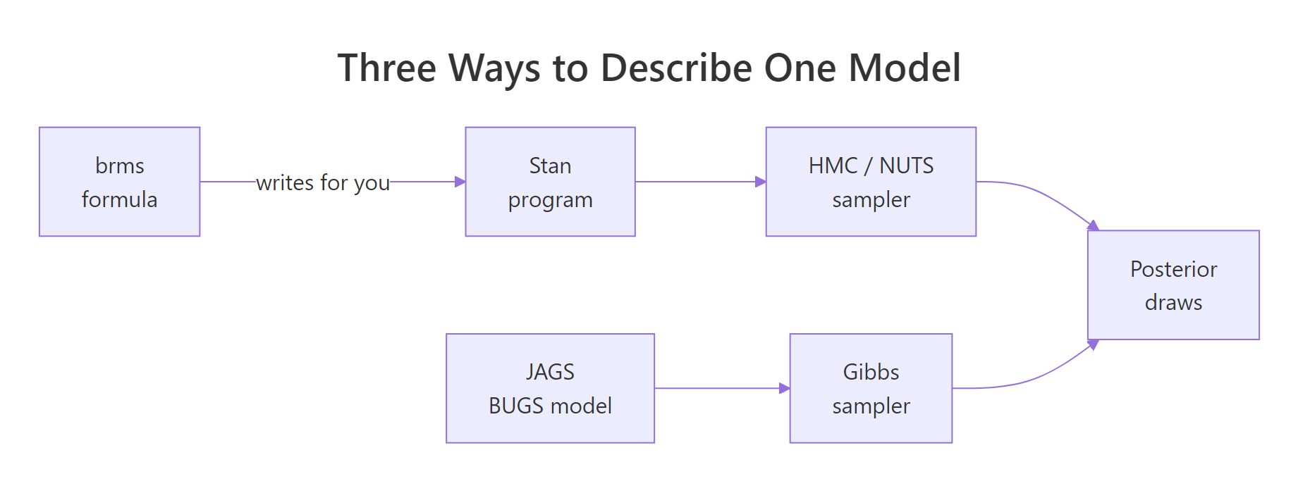
Figure 1: brms writes Stan for you, while JAGS runs its own Gibbs engine. All roads end at posterior draws.
To compare the three fairly, we need one concrete model. Let's simulate a simple linear regression where the true intercept is 2 and the true slope is 0.5, then look at the data and fit an ordinary least-squares line as a reference point.
Least squares recovers a slope of 0.48, close to the true 0.5. That is a single best-guess line with no uncertainty attached. The Bayesian version returns a posterior for the slope instead. Here is how you would ask each package for it.
With brms, the model is the same formula you gave lm(), plus a prior and a family. You never write any Stan code.
library(brms)

fit_brms <- brm(
  y ~ x,                                     # same formula you would give lm()
  data   = d,
  family = gaussian(),
  prior  = prior(normal(0, 1), class = "b") # prior on the slope
)

summary(fit_brms)   # posterior means, 95% credible intervals, and convergence diagnostics
With Stan, you write a small program with three blocks: the data it expects, the parameters to estimate, then the model that connects them. You then call it from R.
// slope_model.stan
data {
  int<lower=1> N;
  vector[N] x;
  vector[N] y;
}
parameters {
  real a;                 // intercept
  real b;                 // slope
  real<lower=0> sigma;    // noise standard deviation
}
model {
  b ~ normal(0, 1);              // prior on the slope
  y ~ normal(a + b * x, sigma);  // likelihood
}
library(rstan)
fit_stan <- stan(
file = "slope_model.stan",
data = list(N = nrow(d), x = d[["x"]], y = d[["y"]])
)
print(fit_stan, pars = c("a", "b", "sigma"))With JAGS, you write a BUGS model. It looks similar to Stan but reads as a set of declarations, and it parameterises the normal by precision rather than standard deviation.
model {
  for (i in 1:N) {
    y[i] ~ dnorm(a + b * x[i], tau)   # tau is precision = 1 / variance
  }
  a   ~ dnorm(0, 0.001)               # vague prior on the intercept
  b   ~ dnorm(0, 1)                   # prior on the slope
  tau ~ dgamma(0.01, 0.01)            # prior on the precision
}
library(rjags)
# model_string holds the model block above, stored as a string
jags <- jags.model(textConnection(model_string),
data = list(N = nrow(d), x = d[["x"]], y = d[["y"]]))
samples <- coda.samples(jags, variable.names = c("a", "b"), n.iter = 2000)
summary(samples)Notice the trade-off. The brms version is three lines and needs no new language. The Stan and JAGS versions are more verbose but let you write relationships that no formula could express.
dnorm(mean, tau) where tau is the precision, equal to 1 divided by the variance. A big tau means small spread. Stan and brms use the standard deviation directly, so watch the switch when you port a model.Is the claim that brms writes Stan for you literally true? Yes. brms has a function that shows you the exact Stan program it builds from your formula, and it runs without fitting anything. Let's look at the data block it generates.
library(brms)

# make_stancode turns a formula into a full Stan program, no Stan coding required
stan_prog <- make_stancode(y ~ x, data = d, family = gaussian())
cat(paste(strsplit(as.character(stan_prog), "\n")[[1]][4:11], collapse = "\n"))
#> data {
#>   int<lower=1> N;  // total number of observations
#>   vector[N] Y;  // response variable
#>   int<lower=1> K;  // number of population-level effects
#>   matrix[N, K] X;  // population-level design matrix
#>   int<lower=1> Kc;  // number of population-level effects after centering
#>   int prior_only;  // should the likelihood be ignored?
#> }
The walk-through: make_stancode() returns the Stan program brms would compile, and we print its data block. That block is Stan code, written for you, from a one-line formula. The interpretation: brms is not a different method from Stan, it is a code generator that writes Stan for you, which is why anything brms fits, Stan can fit too.
Try it: Get the 95% confidence interval for the slope from the lm() fit with confint(), so you have a frequentist interval to compare against a Bayesian one later.
Click to reveal solution
Explanation: The frequentist interval runs from 0.38 to 0.58. A Bayesian credible interval from any of the three packages will land in a similar place for this simple model, but it carries a direct probability reading: the slope is 95% likely to be inside it.
What sampler runs under the hood, and why does it matter?
When the posterior is too complex for a grid, the packages approximate it by drawing thousands of samples from it. This is Markov chain Monte Carlo, or MCMC. The two big families of sampler explain most of the practical differences between the packages.
JAGS uses Gibbs sampling. It updates one parameter at a time, drawing each from its distribution given the current values of all the others. It is simple and needs no gradients, but it can get stuck taking tiny steps when parameters are correlated. Stan and brms use Hamiltonian Monte Carlo, or HMC, with a variant called the No-U-Turn Sampler. HMC uses the gradient of the posterior to propose long, informed jumps, so it explores correlated, high-dimensional models far more efficiently.
To make MCMC concrete, let's build the simplest sampler by hand, a random-walk Metropolis sampler, for the slope of our regression. We hold the intercept and noise at their least-squares values and let the slope wander. At each step we propose a small move, then accept it with a probability set by how much better or worse it makes the posterior.
$$\alpha = \min\left(1, \; \frac{p(\theta' \mid y)}{p(\theta \mid y)}\right)$$
Where $\theta'$ is the proposed value and $\theta$ is the current value. If the proposal is better the ratio exceeds 1 and we always accept; if it is worse we accept it only sometimes. If you are not interested in the mechanics, skip to the output, the numbers are all you need.
The walk-through: we started the slope at 0, proposed a nudge each iteration, and kept or rejected it based on the posterior ratio. After discarding warmup, the retained samples are draws from the posterior of the slope. The interpretation: the posterior mean is 0.479, matching both the true 0.5 and the least-squares estimate, and about 47% of proposals were accepted. This hand-rolled loop is exactly the kind of work JAGS, Stan, and brms automate for you, only far more efficiently.
A picture helps. Plotting the chain over time shows it wandering around the posterior rather than drifting, which is the sign of a healthy sampler.
Not all samples are worth the same. Because each draw is close to the one before it, the chain carries less information than its raw count suggests. The effective sample size measures how many truly independent draws you effectively have.
The interpretation: 7000 raw draws are worth only about 1319 independent ones here, because a plain random walk takes small, correlated steps. This is precisely the weakness HMC fixes: by using gradients to take long, decorrelated steps, Stan and brms turn the same wall-clock time into many more effective samples, especially as models grow.
Try it: Rerun the sampler with a larger proposal standard deviation of 0.20 instead of 0.05, and report the acceptance rate. Reuse the logpost function from above.
Click to reveal solution
Explanation: Bigger jumps overshoot the posterior more often, so only 14% are accepted. Tuning this step size by hand is fiddly, which is another reason HMC and its auto-tuning are so valuable.
Which package should you use, and how do they compare?
Now that you know what the three packages do and how they sample, the choice comes down to your model and your priorities. Here is the practical comparison.
| Dimension | brms | Stan (rstan) | JAGS (rjags) |
|---|---|---|---|
| How you specify a model | lme4-style formula | Stan program | BUGS model |
| Sampler | HMC / NUTS | HMC / NUTS | Gibbs + others |
| Learning curve | Gentle for R users | Steep | Moderate |
| Discrete parameters | No | No | Yes |
| Speed on hard models | Fast | Fast | Slower |
| What you install | A C++ toolchain | A C++ toolchain | The JAGS program |
Two rows deserve a note. First, both brms and Stan need a C++ compiler because Stan translates your model to C++ and compiles it, which adds a one-time build step per model. JAGS ships as its own program that R talks to, so there is nothing to compile. Second, only JAGS can sample discrete unknowns directly, such as a hidden class label, because HMC needs a continuous, differentiable surface to compute gradients on.
The decision usually follows a short path.
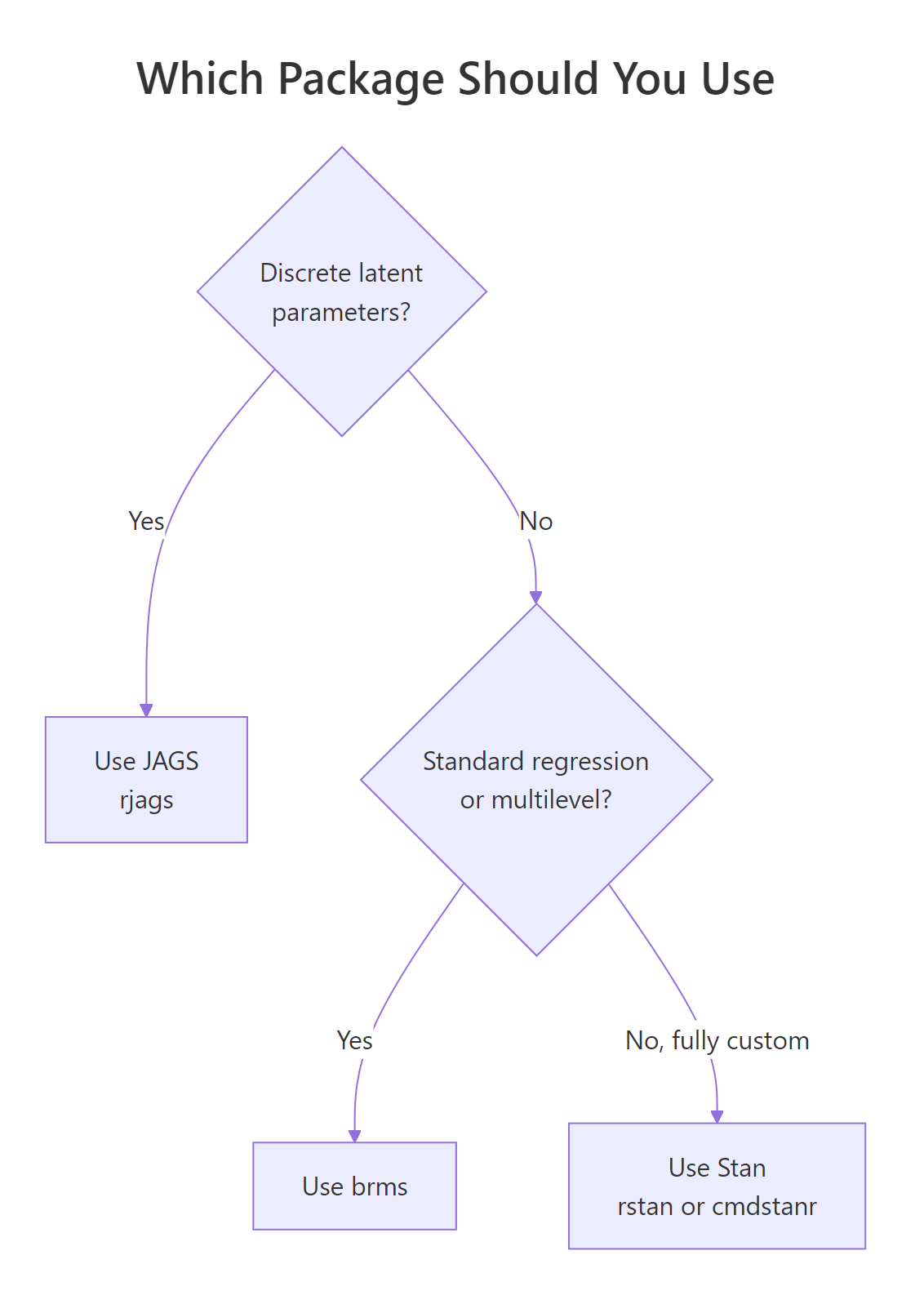
Figure 2: A quick decision path for picking the right Bayesian package.
- Reach for brms when your model is a regression, a generalised linear model, or a multilevel model, which covers the large majority of applied work, and you get Stan's speed without writing Stan.
- Drop down to Stan when the formula interface cannot express your model, for example a custom likelihood or an unusual parameter constraint, or when you want maximum control and speed.
- Choose JAGS when your model has discrete latent parameters, or when you are working from existing BUGS or JAGS code and translating it would cost more than it is worth.
Whatever you pick, the output is the same shape: a set of posterior draws that you summarise the same way. Here is the 95% credible interval for our slope, straight from the Metropolis draws.
The interpretation: given the data and prior, there is a 95% probability the slope lies between 0.44 and 0.53. brms, Stan, and JAGS would each hand you draws you summarise with this very line. The package decides how you write and run the model; it does not change how you read the answer.
Try it: From the same draws, compute the posterior probability that the slope is greater than 0.5.
Click to reveal solution
Explanation: About 17% of the posterior mass sits above 0.5. Turning a question into a probability by counting draws is one of the everyday joys of Bayesian work, and it looks identical no matter which package produced the draws.
FAQ
Do I need to install anything special to use them? brms and Stan both need a C++ toolchain, called Rtools on Windows, because Stan compiles each model. JAGS is a separate program you install first, and then the rjags package talks to it. brms is usually the smoothest to set up on a fresh machine because a single package install pulls in what it needs.
Is brms just Stan underneath? Yes. brms translates your formula into a Stan program and hands it to Stan to fit, as the generated-code example above showed. Anything brms can fit, Stan can fit, but not the other way around, because raw Stan can express models no formula can.
Can JAGS do everything Stan can? Not quite. JAGS can sample discrete unknown parameters that Stan cannot, which is a real advantage for some mixture and hidden-state models. But JAGS mixes more slowly on large, correlated models, where Stan's gradient-based sampler pulls ahead.
Which one is fastest? For most non-trivial models, Stan and brms are faster in effective samples per second because HMC explores the posterior more efficiently. JAGS can be competitive on small models with conjugate structure where Gibbs steps are cheap.
Do I have to learn the Stan language to use brms? No. You can go a long way with brms writing only R formulas. Learning to read Stan helps you understand and debug what brms generates, but it is not required to get results.
What about rstanarm, PyMC, or NIMBLE? rstanarm is a sibling of brms with pre-compiled models for common regressions, so it skips the compile step but supports fewer model types. PyMC is the popular Python equivalent of this space, and NIMBLE is a BUGS-compatible R package that compiles its samplers for extra speed. They are worth knowing, but brms, Stan, and JAGS remain the most common starting points in R.
Practice Exercises
These two problems reuse the ideas above. Both run in your browser with base R.
Exercise 1: Posterior for a proportion
You ran a small test and observed 18 successes out of 25 trials. Using a uniform prior on the success probability, grid-approximate the posterior mean and 95% credible interval. Use dbinom() for the likelihood over a grid of probabilities from 0 to 1.
Click to reveal solution
Explanation: The posterior mean of 0.70 is close to the raw rate 18/25 = 0.72, pulled slightly toward 0.5 by the prior, and the wide interval reflects how little 25 trials tell you. This is the same grid recipe from the first section, applied to a proportion instead of a mean.
Exercise 2: Sample an unknown mean
Return to the 12 reaction times in y. Write a Metropolis sampler for the unknown mean, using a known noise standard deviation of 0.25 and a Normal(2, 0.5) prior, then report the posterior mean and 95% credible interval. Compare your answer to the grid result from the first section.
Click to reveal solution
Explanation: The sampler lands on a posterior mean of 2.10 with a 95% interval of 1.96 to 2.23, matching the grid answer from the first section almost exactly. Two different methods, one posterior, which is the whole point: the tool is a means to the same end.
Summary
The three packages are front ends to the same idea. Pick based on how you want to write the model and what it needs to do.
| Package | Write a model as | Best when |
|---|---|---|
| brms | A one-line R formula | Regression, GLM, or multilevel work (most cases) |
| Stan | A Stan program | Custom likelihoods, unusual constraints, top speed |
| JAGS | A BUGS model | Discrete latent parameters or legacy BUGS code |
The one-line rule of thumb: default to brms, drop to Stan when the formula cannot express your model, and reach for JAGS when you need discrete parameters or already have BUGS code. Whichever you choose, you read the result the same way, as posterior draws you summarise into means, intervals, and probabilities.
References
- Burkner, P. (2017). brms: An R Package for Bayesian Multilevel Models Using Stan. Journal of Statistical Software. Link The canonical brms paper: what the formula interface can express and how it becomes Stan code.
- brms package documentation on CRAN. Link The CRAN reference for brms functions, including the
make_stancodecall used above. - Stan Development Team. Stan Reference Manual. Link The definitive guide to the Stan language and its HMC sampler.
- Plummer, M. JAGS: Just Another Gibbs Sampler. Project page. Link The JAGS project home: downloads and the BUGS modelling syntax.
- rjags package documentation on CRAN. Link How to drive JAGS from R with the
rjagscalls shown above. - Ponisio, L. et al. (2021). JAGS, NIMBLE, Stan: a detailed comparison among Bayesian MCMC software. arXiv. Link A head-to-head benchmark if you want numbers behind the speed comparison.
- Kurz, A. S. Doing Bayesian Data Analysis in brms and the tidyverse. Link A full course that fits real models in brms, a good next step after this page.
- Jumping Rivers. Should I learn Stan? Link A short take on when dropping from brms to raw Stan is worth it.
Continue Learning
- brms in R: the parent tutorial, fitting Bayesian regressions with the formula interface end to end.
- Stan in R: write and fit your first Stan model when brms is not enough.
- MCMC in R: build a Metropolis-Hastings sampler from scratch to understand what these engines automate.
- MCMC Diagnostics in R: the four checks that tell you whether your chains have converged.