Bayesian Factor Analysis in R with blavaan

Bayesian factor analysis uncovers the hidden factors behind a set of correlated measurements, and instead of a single number for each factor loading it hands you a full probability distribution, so you see both the estimate and how sure you can be about it. In R, the blavaan package fits these models with almost the same syntax as lavaan, so if you can write a classical factor model you can write a Bayesian one.

By Selva Prabhakaran · August 2026

Code examples run against R 4.6.0

This tutorial builds the idea from the ground up. You will simulate data with a known hidden structure and run it right here on the page, watch a classical factor analysis recover that structure as bare point estimates, and then upgrade to blavaan to get the full posterior: loadings with credible intervals, convergence checks, and a look at how much your priors actually change the answer. The hands-on intuition uses base R, so nothing needs installing to follow along. The blavaan sections are marked to run in your own R install, because they lean on the Stan engine.

What is factor analysis, and where do the hidden factors come from?

Suppose you gave 250 students six short tests. You cannot measure "math ability" with a ruler, but if it exists, the math-flavored tests should rise and fall together, and so should the verbal ones. Factor analysis works backward from those correlations to the hidden abilities that could have produced them. Let us build exactly that situation, so we know the true answer before we look.

We will create two hidden factors, a math factor and a verbal factor, and let them be mildly correlated (real abilities usually are). Then we build six observed test scores: three driven mostly by math, three driven mostly by verbal, each with its own random noise. Because we made the data, we know the truth going in.

RSimulate six scores from two hidden factors

set.seed(2024) n <- 250 math <- rnorm(n) verbal <- 0.4 * math + sqrt(1 - 0.4^2) * rnorm(n) # verbal correlates ~0.4 with math m1 <- 0.80 * math + rnorm(n, 0, 0.6) m2 <- 0.70 * math + rnorm(n, 0, 0.6) m3 <- 0.60 * math + rnorm(n, 0, 0.6) v1 <- 0.80 * verbal + rnorm(n, 0, 0.6) v2 <- 0.70 * verbal + rnorm(n, 0, 0.6) v3 <- 0.60 * verbal + rnorm(n, 0, 0.6) scores <- data.frame(m1, m2, m3, v1, v2, v3) dim(scores) #> [1] 250 6 round(head(scores, 3), 2) #> m1 m2 m3 v1 v2 v3 #> 1 1.25 0.56 0.56 1.86 2.91 1.35 #> 2 -0.06 0.71 -0.02 0.92 0.13 0.11 #> 3 0.39 1.08 -0.61 -0.62 1.06 0.01

The block created a data frame of 250 rows and 6 columns, one column per test. Notice that the two factors themselves, math and verbal, are not in the data frame. That is the whole point: in real life you never observe the factor, only the noisy scores it produced. The diagram below shows the machine we just built.

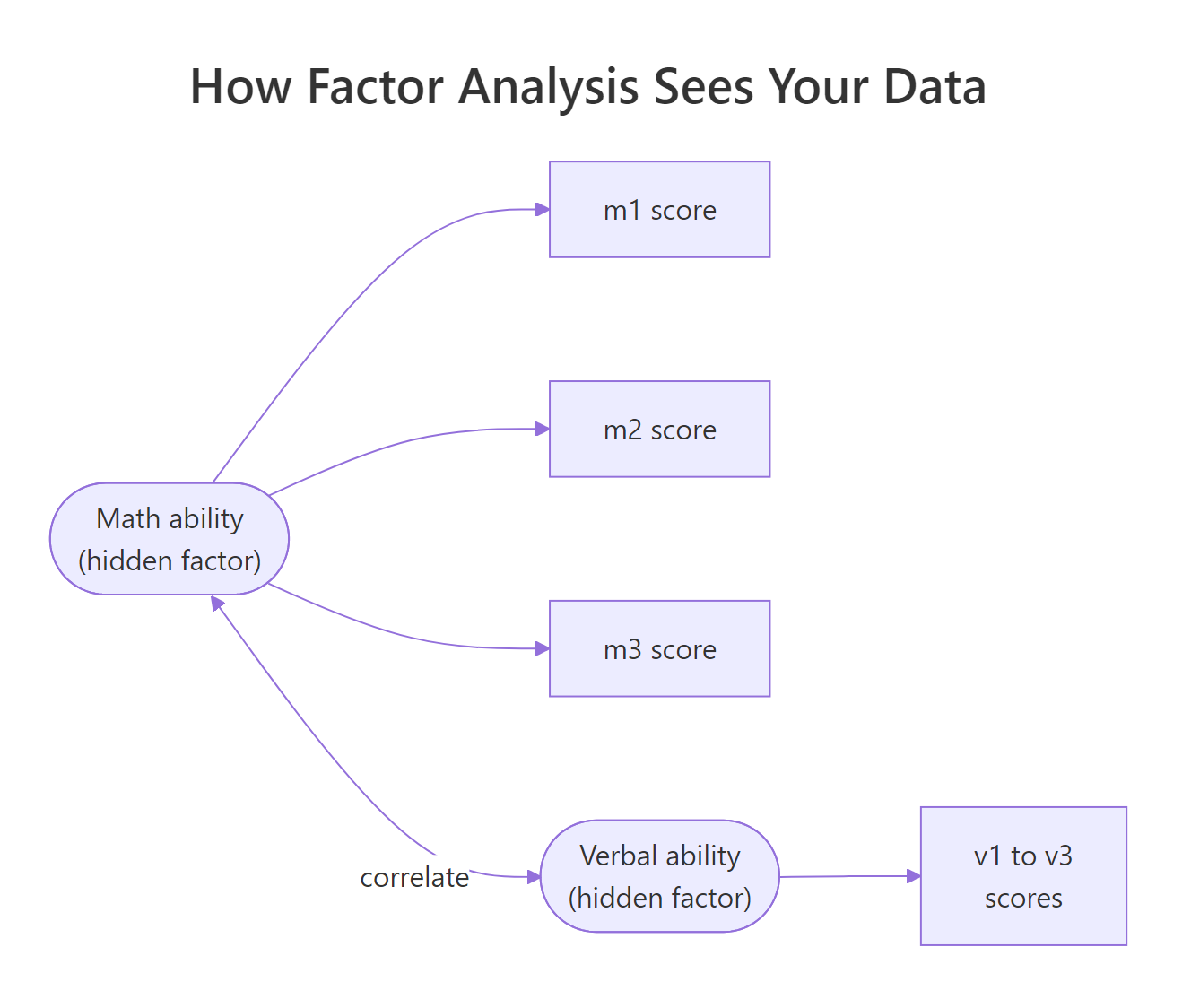
How factor analysis sees your data, with each hidden factor driving its own scores

Figure 1: Each hidden factor drives its own set of observed scores, and the two factors can correlate.

If the hidden factors are real, their fingerprints show up as correlations. Scores driven by the same factor should correlate strongly with each other and weakly with scores from the other factor. Let us look at the correlation matrix and check.

RRead the correlation fingerprints

round(cor(scores), 2) #> m1 m2 m3 v1 v2 v3 #> m1 1.00 0.66 0.67 0.33 0.36 0.28 #> m2 0.66 1.00 0.61 0.28 0.36 0.23 #> m3 0.67 0.61 1.00 0.28 0.32 0.26 #> v1 0.33 0.28 0.28 1.00 0.59 0.52 #> v2 0.36 0.36 0.32 0.59 1.00 0.47 #> v3 0.28 0.23 0.26 0.52 0.47 1.00

Read the matrix in two blocks. The top-left three-by-three corner (the m tests) shows correlations around 0.6, and so does the bottom-right corner (the v tests). The off-diagonal block linking m tests to v tests sits lower, around 0.3. That two-block pattern is the visible trace of two hidden factors. A quick heatmap makes the blocks jump out.

RPicture the correlation blocks

cols <- colorRampPalette(c("white", "steelblue"))(20) image(1:6, 1:6, cor(scores)[, 6:1], col = cols, axes = FALSE, xlab = "", ylab = "", main = "Correlations light up in two blocks") axis(1, at = 1:6, labels = colnames(scores)) axis(2, at = 1:6, labels = rev(colnames(scores)))

The darker the square, the stronger the correlation. Two dark blocks appear along the diagonal, one for the math tests and one for the verbal tests, with paler squares linking the two groups. Factor analysis is the formal tool that turns this eyeballed pattern into numbers.

Key Insight

Correlations are the clue; factors are the explanation. Factor analysis never measures the hidden abilities directly. It reads the pattern of correlations and works backward to the smallest set of hidden factors that could plausibly have produced that pattern.

The word "Bayesian" adds one more idea on top. A Bayesian analysis starts with a prior, a statement of what you believe before seeing the data, then updates it with the data to produce a posterior, a full distribution of plausible values. If that language is new, the MCMC in R and Grid Approximation in R tutorials build it from scratch. Here you only need the one-line version: Bayesian factor analysis returns a distribution for every loading, not a single number.

Try it: Confirm the block pattern yourself. Compute the correlation between two math tests (m1 and m2) and between a math test and a verbal test (m1 and v1), and see which is larger.

RYour turn: compare two correlations

# Fill in the two cor() calls, then run. ex_within <- 0 # cor of m1 and m2 (same factor) ex_between <- 0 # cor of m1 and v1 (different factors)

Click to reveal solution

RCompare two correlations solution

ex_within <- cor(scores$m1, scores$m2) ex_between <- cor(scores$m1, scores$v1) round(c(within = ex_within, between = ex_between), 2) #> within between #> 0.66 0.33

Explanation: Two tests driven by the same factor correlate about twice as strongly (0.66) as two tests from different factors (0.33). That gap is exactly what factor analysis exploits.

What does classical factor analysis give you, and what does it leave out?

Before fitting anything, a factor analysis asks one question: how many factors? A common quick check counts how many eigenvalues of the correlation matrix exceed 1. Each eigenvalue measures how much shared variance one direction captures, and a value above 1 means that direction explains more than a single test's worth of variance. Let us compute them.

RCount the factors with eigenvalues

ev <- eigen(cor(scores))$values round(ev, 2) #> [1] 3.09 1.27 0.54 0.41 0.37 0.31

Two eigenvalues sit above 1 (3.09 and 1.27) and the rest fall well below, so the data point clearly to two factors. That matches how we built it. Now we run a classical factor analysis. Base R ships factanal(), which fits a factor model by maximum likelihood and rotates the result so each test loads cleanly on one factor.

RFit a classical factor analysis

fa <- factanal(scores, factors = 2, rotation = "promax") print(fa$loadings, cutoff = 0.3) #> #> Loadings: #> Factor1 Factor2 #> m1 0.842 #> m2 0.776 #> m3 0.800 #> v1 0.838 #> v2 0.686 #> v3 0.648 #> #> Factor1 Factor2 #> SS loadings 1.961 1.593 #> Proportion Var 0.327 0.265 #> Cumulative Var 0.327 0.592

The loadings table splits perfectly. The three m tests load on Factor1 (values around 0.8) and the three v tests load on Factor2, with the small cross-loadings hidden by the 0.3 cutoff. A loading is just the strength of the link between a test and its factor, on a scale where 1 is a perfect match and 0 is no relationship. Together the two factors explain about 59 percent of the total variance (the cumulative variance row).

This is a good result, and for many jobs it is enough. But look closely at what you got: one number per loading, and nothing else. There is no sense of how firm the 0.842 is. If you collected a fresh sample of 250 students, would it come back as 0.84, or could it be 0.72 or 0.95? The point estimate cannot say. The diagram below frames the gap this tutorial closes.

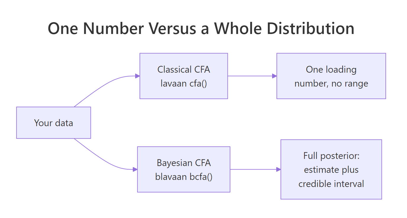
Classical CFA returns one number per loading while Bayesian CFA returns a full posterior

Figure 2: Classical CFA returns one number per loading; Bayesian CFA returns a full posterior with a credible interval.

Warning

A single loading number hides how sure you are. Classical factor analysis hands you one value per loading with no built-in sense of how much it might wobble in a new sample. Two studies can both report a 0.84 loading while one is rock solid and the other is barely distinguishable from zero.

Try it: factanal() also reports uniquenesses, the share of each test's variance that its factor does not explain. Pull them out of the fitted object with fa$uniquenesses and find the largest one.

RYour turn: find the largest uniqueness

# The uniquenesses live in fa$uniquenesses. # Round them, then find which test has the biggest.

Click to reveal solution

RLargest uniqueness solution

round(fa$uniquenesses, 2) #> m1 m2 m3 v1 v2 v3 #> 0.28 0.40 0.37 0.34 0.47 0.58

Explanation: v3 has the largest uniqueness (0.58), meaning its verbal factor explains the least of its variance. High uniqueness marks a test that is only loosely tied to its factor.

How do you fit a Bayesian factor analysis with blavaan?

Now we switch from exploring to confirming. So far factanal() discovered the structure for us. In a confirmatory factor analysis you state the structure up front, which m tests belong to math and which v tests belong to verbal, and let the model estimate the loadings for that fixed design. The lavaan package writes this structure with a compact syntax where =~ reads as "is measured by".

The classical confirmatory fit is a natural stepping stone, because blavaan reuses the exact same model string. First the frequentist version with lavaan's cfa().

Note

blavaan needs a full local R setup. The blavaan package fits its models with the Stan engine, which compiles and samples outside the lightweight editor on this page. Run every blavaan block from here on in your own R installation, where blavaan, lavaan, and rstan are installed.

library(lavaan)

model <- '
  math   =~ m1 + m2 + m3
  verbal =~ v1 + v2 + v3
'

fit_ml <- cfa(model, data = scores, std.lv = TRUE)
parameterEstimates(fit_ml)[1:6, c("lhs", "op", "rhs", "est", "se", "pvalue")]
#>      lhs op rhs   est    se pvalue
#> 1   math =~  m1 0.856 0.056      0
#> 2   math =~  m2 0.707 0.052      0
#> 3   math =~  m3 0.671 0.048      0
#> 4 verbal =~  v1 0.765 0.061      0
#> 5 verbal =~  v2 0.639 0.053      0
#> 6 verbal =~  v3 0.506 0.050      0

The std.lv = TRUE argument fixes each factor's variance to 1, which puts all six loadings on the same readable scale. The frequentist fit gives an estimate (est), a standard error (se), and a p-value for each loading. That is more than factanal() offered, but the standard error still summarizes uncertainty as one number and leans on a large-sample approximation. The Bayesian fit replaces that approximation with the real thing.

To go Bayesian, change cfa() to bcfa(). The model string, the data, and std.lv = TRUE stay identical. The new arguments describe the sampler: how many chains to run, how many warmup iterations to discard, how many to keep, and a seed so the run is reproducible.

library(blavaan)

fit <- bcfa(model, data = scores, std.lv = TRUE,
            n.chains = 2, burnin = 500, sample = 500,
            seed = 1234, bcontrol = list(cores = 1))
summary(fit)
#> blavaan 0.5.10 ended normally after 500 iterations
#> 
#>   Estimator                                      BAYES
#>   Optimization method                             MCMC
#>   Number of model parameters                        13
#> 
#>   Number of observations                           250
#> 
#>   Statistic                                 MargLogLik         PPP
#>   Value                                      -1728.171       0.630
#> 
#> Parameter Estimates:
#> 
#> Latent Variables:
#>                    Estimate  Post.SD pi.lower pi.upper     Rhat    Prior
#>   math =~
#>     m1                0.866    0.059    0.754    0.986    1.000    normal(0,10)
#>     m2                0.716    0.056    0.612    0.826    1.001    normal(0,10)
#>     m3                0.679    0.051    0.579    0.781    1.000    normal(0,10)
#>   verbal =~
#>     v1                0.775    0.062    0.657    0.901    0.999    normal(0,10)
#>     v2                0.647    0.059    0.531    0.755    0.998    normal(0,10)
#>     v3                0.511    0.053    0.409    0.620    0.999    normal(0,10)
#> 
#> Covariances:
#>                    Estimate  Post.SD pi.lower pi.upper     Rhat    Prior
#>   math ~~
#>     verbal            0.510    0.063    0.386    0.629    0.999     lkj_corr(1)
#> 
#> Variances:
#>                    Estimate  Post.SD pi.lower pi.upper     Rhat    Prior
#>    .m1                0.283    0.050    0.191    0.386    0.999 gamma(1,.5)[sd]
#>    .m2                0.343    0.043    0.267    0.435    0.998 gamma(1,.5)[sd]
#>    .m3                0.272    0.036    0.206    0.342    0.998 gamma(1,.5)[sd]
#>    .v1                0.378    0.065    0.252    0.503    1.000 gamma(1,.5)[sd]
#>    .v2                0.314    0.049    0.223    0.411    1.000 gamma(1,.5)[sd]
#>    .v3                0.368    0.043    0.293    0.458    0.998 gamma(1,.5)[sd]
#>     math              1.000
#>     verbal            1.000

There is a lot here, so take it one piece at a time. Under Latent Variables you get the loadings, one row per test. The Estimate column is the posterior mean loading, and it lands right where we built the data: about 0.87, 0.72, 0.68 for the math tests and 0.78, 0.65, 0.51 for the verbal tests. The model recovered the hidden structure. Under Covariances, the math ~~ verbal row estimates the correlation between the two factors at 0.510, in the same moderate range as the 0.4 we baked in.

The three columns that classical factor analysis could never give you are Post.SD, pi.lower, and pi.upper. Together they turn each loading from a lone number into a range, which the next section reads in detail. The Rhat column and the PPP value near the top are health checks we cover after that.

Behind the scenes, blavaan drew a thousand plausible parameter sets from the posterior using Markov chain Monte Carlo, the same sampling engine behind Bayesian linear regression. Every number in the summary is a summary of those draws.

Try it: The summary is formatted for reading, but you often want the loadings as a plain table you can compute on. Extract them with parameterEstimates(fit) and keep only the loading rows (the ones where op equals "=~").

# parameterEstimates(fit) returns one row per parameter.
# Keep only the rows where op == "=~".

Click to reveal solution

pe <- parameterEstimates(fit)
pe[pe$op == "=~", ]
#>      lhs op rhs   est
#> 1   math =~  m1 0.866
#> 2   math =~  m2 0.716
#> 3   math =~  m3 0.679
#> 4 verbal =~  v1 0.775
#> 5 verbal =~  v2 0.647
#> 6 verbal =~  v3 0.511

Explanation: parameterEstimates() returns every model parameter as a tidy data frame. Filtering to op == "=~" leaves just the six loadings, ready to plot or compare.

How do you read the posterior loadings and credible intervals?

The payoff of going Bayesian is the credible interval. For the loading of m1, the summary reported a posterior mean of 0.866 with a 95 percent interval from pi.lower 0.754 to pi.upper 0.986. Read that as a direct probability statement: given the data and priors, there is a 95 percent probability that the true loading of m1 lies between 0.754 and 0.986.

That is exactly the sentence people wish they could say about a classical confidence interval but technically cannot. A confidence interval is a statement about a procedure repeated across many hypothetical samples, not about this one number. The credible interval is about your actual result.

Key Insight

A credible interval says what you actually want to hear. A 95 percent credible interval means there is a 95 percent probability the loading lies inside it, given your data and priors. That is the plain-language claim people mistakenly attach to classical confidence intervals.

Two loadings can share the same estimate yet carry very different certainty, and the interval width is what tells them apart. A narrow interval means the data pin the loading down; a wide interval means the loading is still fuzzy. In our fit every loading interval sits comfortably above zero, so every test is clearly tied to its factor.

If you want the formal picture, the model behind all of this is one small equation per test. Each observed score is its factor times a loading, plus its own noise:

$$x_i = \lambda_i \, \xi + \varepsilon_i$$

Where:

$x_i$ = the observed score on test $i$
$\lambda_i$ = the loading, how strongly the factor drives test $i$
$\xi$ = the hidden factor score for a person
$\varepsilon_i$ = the unique noise in test $i$ that the factor does not explain

If the math is not your thing, skip it: the loadings and their credible intervals in the summary are all you need to act on.

Try it: Count how many of the six loadings have a posterior mean above 0.6, a rough line for a "strong" loading. Reuse the pe table from the last exercise.

# The loading estimates are pe$est where pe$op == "=~".
# Count how many exceed 0.6.

Click to reveal solution

load_est <- pe$est[pe$op == "=~"]
sum(load_est > 0.6)
#> [1] 5

Explanation: Five of the six loadings clear 0.6. Only v3, at 0.511, falls short, matching the high uniqueness we found for it earlier.

How do you check the chains converged and the model fits?

Before trusting any of those numbers, you must confirm the sampler actually worked. Markov chain Monte Carlo explores the posterior by wandering through it, and you run several chains from different starting points. If they all end up describing the same distribution, you can trust the summary. The diagnostic that measures this is Rhat: it compares the variation within each chain to the variation between chains, and it should sit at or just above 1.00. A common rule is that every Rhat must be below 1.01.

round(blavInspect(fit, "rhat"), 3)
#>     math=~m1     math=~m2     math=~m3   verbal=~v1   verbal=~v2   verbal=~v3       m1~~m1 
#>        1.000        1.001        1.000        0.999        0.998        0.999        0.999 
#>       m2~~m2       m3~~m3       v1~~v1       v2~~v2       v3~~v3 math~~verbal 
#>        0.998        0.998        1.000        1.000        0.998        0.999

Every value is essentially 1.00, so the chains converged and the estimates are safe to read. A companion number, the effective sample size from blavInspect(fit, "neff"), tells you how many independent draws you effectively have; here it runs into the hundreds for every parameter, which is plenty.

Warning

Never read the estimates until the chains have converged. If any Rhat is well above 1.01, the sampler has not settled and the numbers in the summary are not yet trustworthy. Check convergence first, interpret second.

Convergence tells you the sampler worked, but not whether the model fits the data. For that, blavaan reports a posterior predictive p-value, or PPP. It simulates fresh data from the fitted model and asks how often that simulated data looks as extreme as your real data. A value near 0.5 means the model reproduces the data well; values near 0 or 1 signal misfit.

fitMeasures(fit, "ppp")
#>  ppp 
#> 0.63

A PPP of 0.63 is comfortably mid-range, so the two-factor model is a good description of the six tests. That makes sense, because two factors are exactly how we built the data.

Try it: Convergence checks are worth automating. Write one line that returns the largest Rhat across all parameters, so you can confirm at a glance that it clears the 1.01 rule.

# blavInspect(fit, "rhat") returns every Rhat.
# Return the largest one.

Click to reveal solution

round(max(blavInspect(fit, "rhat")), 3)
#> [1] 1.001

Explanation: The worst Rhat in the whole model is 1.001, well under 1.01, so every chain converged. Wrapping the check in max() scales to models with hundreds of parameters.

How much do your priors change the result?

Every Bayesian model starts from priors, and blavaan picks sensible defaults so you rarely have to. You can see them all with dpriors().

dpriors()
#>                nu             alpha            lambda              beta             theta 
#>    "normal(0,32)"    "normal(0,10)"    "normal(0,10)"    "normal(0,10)" "gamma(1,.5)[sd]" 
#>               psi               rho             ibpsi               tau 
#> "gamma(1,.5)[sd]"       "beta(1,1)" "wishart(3,iden)"   "normal(0,1.5)"

The one that matters most for factor analysis is lambda, the prior on the loadings, set to normal(0, 10). A normal centered at 0 with a standard deviation of 10 is very wide: it says a loading could plausibly be almost anything in the usual range, so the data do nearly all the talking. Priors like this are called weakly informative. The residual variances (theta) and factor variances (psi) get a gamma prior that keeps them positive.

Do the priors actually move the answer? Let us find out by refitting with a much tighter prior on the loadings, normal(0, 1), using the dp argument, and comparing the loadings side by side.

fit_info <- bcfa(model, data = scores, std.lv = TRUE,
                 dp = dpriors(lambda = "normal(0,1)"),
                 n.chains = 2, burnin = 500, sample = 500,
                 seed = 4321, bcontrol = list(cores = 1))

pe_d <- parameterEstimates(fit)
pe_i <- parameterEstimates(fit_info)
ld   <- pe_d$op == "=~"
data.frame(loading     = paste0(pe_d$lhs, pe_d$op, pe_d$rhs)[ld],
           default     = round(pe_d$est[ld], 3),
           informative = round(pe_i$est[ld], 3))
#>      loading default informative
#> 1   math=~m1   0.866       0.859
#> 2   math=~m2   0.716       0.712
#> 3   math=~m3   0.679       0.675
#> 4 verbal=~v1   0.775       0.768
#> 5 verbal=~v2   0.647       0.641
#> 6 verbal=~v3   0.511       0.507

The loadings barely budge. Tightening the prior tenfold shifts every estimate by less than 0.01. With 250 rows of data, the likelihood overwhelms the prior, so the exact prior choice hardly matters here. That is the reassuring case, and it is common with a healthy sample size.

Tip

Check prior sensitivity whenever your sample is small. With plenty of data the likelihood dominates and the prior barely matters, as you just saw. When data are scarce, refit with both a tighter and a looser prior and watch how much the answer moves before you trust it.

Try it: Quantify how little changed. Compute the largest absolute difference between the default and informative loadings, reusing the pe_d, pe_i, and ld objects from the last block.

# Compare pe_d$est[ld] with pe_i$est[ld].
# Report the biggest absolute difference.

Click to reveal solution

round(max(abs(pe_d$est[ld] - pe_i$est[ld])), 3)
#> [1] 0.007

Explanation: The largest single change is 0.007, tiny on a loading scale where 1 is a perfect link. The two priors lead to practically the same conclusions.

Practice Exercises

These combine several ideas from the tutorial. Each solution runs in your own R session on top of the fit object you built above. Use fresh variable names so you do not overwrite the tutorial's objects.

Exercise 1: Report the factor correlation with certainty

A key question in factor analysis is how related the factors are. Pull the posterior mean correlation between math and verbal from the fitted model, then find its 95 percent credible interval in the summary output and state whether the interval excludes zero.

# The factor correlation is the math ~~ verbal row of parameterEstimates(fit).
# Its credible interval (pi.lower, pi.upper) is in summary(fit).

# Write your code below:

Click to reveal solution

pe <- parameterEstimates(fit)
round(pe$est[pe$op == "~~" & pe$lhs == "math" & pe$rhs == "verbal"], 2)
#> [1] 0.51

Explanation: The posterior mean correlation is 0.51. The summary reported its 95 percent credible interval as 0.386 to 0.629, which stays well above zero, so the two factors are clearly and reliably related rather than independent.

Exercise 2: Prove a wrong model with a fit check

A CFA can only be trusted if you check that the structure fits. Fit a deliberately wrong one-factor model that forces all six tests onto a single factor g, then compare its posterior predictive p-value to the correct two-factor model. Decide which model the data prefer.

# Build a one-factor model:  g =~ m1 + m2 + m3 + v1 + v2 + v3
# Fit it with bcfa(..., std.lv = TRUE, seed = 777)
# Compare fitMeasures(fit, "ppp") with fitMeasures(fit_1f, "ppp")

# Write your code below:

Click to reveal solution

model_1f <- ' g =~ m1 + m2 + m3 + v1 + v2 + v3 '
fit_1f <- bcfa(model_1f, data = scores, std.lv = TRUE,
               n.chains = 2, burnin = 500, sample = 500,
               seed = 777, bcontrol = list(cores = 1))

cat("two-factor ppp:", round(fitMeasures(fit, "ppp"), 2), "\n")
cat("one-factor ppp:", round(fitMeasures(fit_1f, "ppp"), 2), "\n")
#> two-factor ppp: 0.63 
#> one-factor ppp: 0

Explanation: The one-factor model has a PPP of 0, a clear sign of misfit, while the two-factor model sits at a healthy 0.63. The data strongly prefer two factors, which is the structure we built. The posterior predictive p-value catches the wrong model that the loadings alone would not.

Summary

Bayesian factor analysis takes the same confirmatory model you would fit with lavaan and returns a full posterior for every parameter, so uncertainty is built in rather than bolted on. Here is the shape of what you learned.

Idea	Classical factor analysis	Bayesian factor analysis (blavaan)
Loading result	one point estimate	posterior mean plus a credible interval
Uncertainty	standard error, large-sample approximation	full posterior distribution, exact
Interval meaning	confidence interval (about the procedure)	credible interval (95 percent probability the value is inside)
Convergence check	not applicable	Rhat below 1.01, effective sample size
Fit check	fit indices	posterior predictive p-value near 0.5
Prior control	none	defaults via dpriors(), overridable

The workflow is short and repeatable: write the measurement model with =~, fit it with bcfa(..., std.lv = TRUE), confirm every Rhat is below 1.01, read the loadings and their credible intervals, sanity-check fit with the posterior predictive p-value, and refit with different priors if your sample is small. If you can do classical CFA, you already know 90 percent of this.

Frequently Asked Questions

Is Bayesian factor analysis the same as confirmatory factor analysis? Confirmatory factor analysis (CFA) is the model: you fix which tests load on which factor and estimate the loadings. Bayesian factor analysis is one way to estimate that model, using priors and posterior sampling instead of maximum likelihood. blavaan fits Bayesian CFA and, more broadly, Bayesian structural equation models.

When should I prefer blavaan over lavaan? Reach for blavaan when you want full uncertainty on every parameter, when your sample is small enough that the large-sample approximations behind classical standard errors get shaky, or when you want to bring in prior knowledge about a loading. For a large clean dataset where you only need point estimates, classical lavaan is faster and often enough.

How many MCMC samples do I need? Enough that every Rhat is at or below 1.01 and the effective sample sizes are in the hundreds or more. The 500 warmup and 500 sampling iterations per chain used here were plenty for this small model, but a larger model with more parameters usually needs more. Always let the diagnostics, not a fixed number, tell you when to stop.

Do the priors bias my results? Weakly informative priors like the default normal(0, 10) on loadings barely move the answer when you have a healthy amount of data, as the prior-sensitivity check in this tutorial showed. Priors matter most with small samples, which is exactly when a little sensible prior information helps rather than hurts. Report a prior sensitivity check so readers can see the effect for themselves.

Why is the first loading not fixed to 1 here? By default blavaan fixes the first loading of each factor to 1 to set the scale. Passing std.lv = TRUE instead fixes each factor's variance to 1 and frees every loading, which is what puts all six loadings on the same readable scale you saw in the summary.

References

Merkle, E. C. and Rosseel, Y. (2018). blavaan: Bayesian Structural Equation Models via Parameter Expansion. Journal of Statistical Software. Link
Merkle, E. C., Fitzsimmons, E., Uanhoro, J., and Goodrich, B. (2021). Efficient Bayesian Structural Equation Modeling in Stan. Journal of Statistical Software. Link
blavaan documentation: Specifying Prior Distributions. Link
blavaan package on CRAN. Link
lavaan project home. Link
lavaan tutorial: Confirmatory Factor Analysis. Link
Stan case study: Bayesian Structural Equation Modeling using blavaan. Link
R documentation for factanal(). Link

Continue Learning

Bayesian Linear Regression in R: the parent tutorial that introduces priors, posteriors, and MCMC on a simpler model before you meet factors.
SEM and CFA in R With lavaan: the frequentist confirmatory factor analysis this tutorial mirrors, with the full lavaan workflow.
Exploratory Factor Analysis in R: how to discover the factor structure when you do not yet know it, the step before confirmation.

Navigate

Bayesian Factor Analysis in R with blavaan

What is factor analysis, and where do the hidden factors come from?

What does classical factor analysis give you, and what does it leave out?

How do you fit a Bayesian factor analysis with blavaan?

How do you read the posterior loadings and credible intervals?

How do you check the chains converged and the model fits?

How much do your priors change the result?

Practice Exercises

Exercise 1: Report the factor correlation with certainty

Exercise 2: Prove a wrong model with a fit check

Summary

Frequently Asked Questions

References

Continue Learning