Bayesian t-Test in R with the BayesFactor Package
A Bayesian t-test compares two ideas, that a real difference exists versus that it does not, and returns a Bayes factor: one number telling you how many times more likely your data is under one idea than the other. In R you run it with ttestBF() from the BayesFactor package, and unlike a p-value it can give you evidence for the "no difference" case.
How is a Bayesian t-test different from a normal t-test?
The ordinary t-test you already know has a blind spot. When it hands back a large p-value, beginners often read that as "there is no difference," but the test never actually says that. It only says the data was not surprising enough to rule out "no difference." A Bayesian t-test fixes that gap by weighing both ideas against each other directly. Let's start from a t-test you can read at a glance.
Here we compare tooth growth in guinea pigs given vitamin C by two delivery methods, orange juice (OJ) or a supplement (VC), using the built-in ToothGrowth data. This whole tutorial uses base R plus one add-on package, so run this first block now.
The p-value is 0.06039. By the usual 0.05 rule that counts as "not significant," so a beginner might conclude the delivery method does not matter. That conclusion is not supported. The p-value measures how surprising this data would be if the two methods were truly identical. It cannot tell you how likely "truly identical" is. That is exactly the question a Bayesian t-test answers.
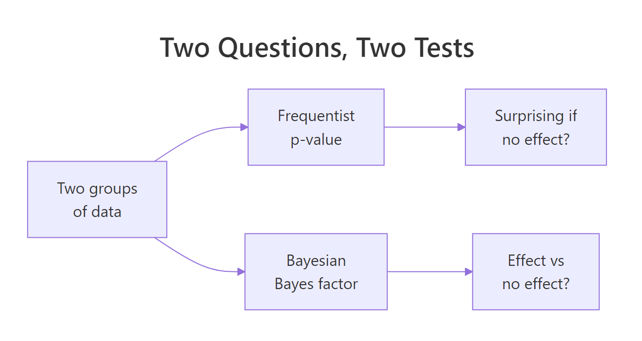
Figure 1: Two tests, two different questions about the same two groups of data.
t.test() block above runs directly in your browser. The BayesFactor blocks below are marked "run this locally" because that package is not built into the in-page runner, so paste them into RStudio to reproduce the exact numbers shown.Try it: Before running any Bayesian test, get a feel for the data. Compute the average tooth length for each supplement group.
Click to reveal solution
Explanation: tapply() splits len by supp and applies mean() to each piece. OJ averages about 3.7 units higher, the same gap the t-test reported.
How do you run a Bayesian t-test with the BayesFactor package?
The BayesFactor package gives you one function, ttestBF(), that covers every flavor of t-test. Install it once with install.packages("BayesFactor"), then load it. The call mirrors t.test(): the same formula = outcome ~ group interface, the same data frame.
Run this locally to score the tooth-growth comparison the Bayesian way.
library(BayesFactor)
bf_tooth <- ttestBF(formula = len ~ supp, data = ToothGrowth)
bf_tooth
#> Bayes factor analysis
#> --------------
#> [1] Alt., r=0.707 : 1.198757
#>
#> Against denominator:
#>   Null, mu1-mu2 = 0
#> ---
#> Bayes factor type: BFindepSample, JZS
Read the printout top to bottom. The line marked [1] is the numerator: the "alternative" idea that a difference exists, with r=0.707 naming the default prior (more on that later). The Against denominator line is the comparison idea: the "null" that the two means are equal, written mu1-mu2 = 0. The number 1.198757 is the Bayes factor comparing them.
That number, usually written $BF_{10}$, is the whole point. Pull it out on its own so you can use it in later code.
extractBF(bf_tooth)$bf
#> [1] 1.198757
A $BF_{10}$ of about 1.2 means your data is only 1.2 times more likely if a difference exists than if it does not. That is a hair above dead even. The Bayesian test and the frequentist p-value of 0.06 agree on the real message here: this data is inconclusive, not proof of "no effect."
install.packages("BayesFactor"). The numbers you get will match this page exactly, because ttestBF() is deterministic.Try it: The value 1.198757 is the evidence for a difference. The evidence for "no difference," written $BF_{01}$, is simply its reciprocal. Compute it.
Click to reveal solution
Explanation: $BF_{01} = 1 / BF_{10} = 0.834$. The data is 0.83 times as likely under "no difference," which is almost the same as 1. Neither side is favored, matching what the p-value hinted.
What does the Bayes factor number actually mean?
A Bayes factor is a ratio of two likelihoods. It asks: how well does the "difference exists" idea ($H_1$) predict the data you saw, compared to the "no difference" idea ($H_0$)?
$$BF_{10} = \frac{P(\text{data} \mid H_1)}{P(\text{data} \mid H_0)}$$
Where:
- $P(\text{data} \mid H_1)$ = how likely your data is if a real difference exists
- $P(\text{data} \mid H_0)$ = how likely your data is if there is no difference
- $BF_{10}$ = the ratio of the two, the number
ttestBF()prints
The reading rule is short. $BF_{10}$ above 1 favors a difference, and the bigger it gets the stronger that support. $BF_{10}$ below 1 favors "no difference." A value near 1 means the data cannot tell the two apart. To turn a raw number into words, statisticians use a labelled scale (the JASP and Jeffreys convention). This helper applies it.
The table walks the whole range. A tiny $BF_{10}$ of 0.05 is real support for the null, our tooth-growth value of 1.2 is barely worth mentioning ("anecdotal"), and a value of 40 is very strong support for a difference. The picture below shows the same scale as a strip you can eyeball.

Figure 2: Reading a Bayes factor, from support for the null on the left to strong support for an effect on the right.
Try it: Suppose a study reports $BF_{10} = 1/3.5$. Label it with the helper you just built.
Click to reveal solution
Explanation: $1/3.5 \approx 0.29$, which lands between $1/10$ and $1/3$, so the scale calls it moderate evidence for the null.
How do you run one-sample and paired Bayesian t-tests?
The same ttestBF() covers the other two designs by swapping arguments. A one-sample test checks whether one group's mean differs from a fixed value, set with mu. Here we ask whether a sleep drug changed sleep at all, testing the extra hours for one drug in the built-in sleep data against mu = 0.
drug2 <- sleep$extra[sleep$group == 2]
ttestBF(x = drug2, mu = 0)
#> Bayes factor analysis
#> --------------
#> [1] Alt., r=0.707 : 10.71554
#>
#> Against denominator:
#>   Null, mu = 0
#> ---
#> Bayes factor type: BFoneSample, JZS
A $BF_{10}$ of about 10.7 is strong evidence that this drug moved sleep away from zero. A paired test is for before-and-after measurements on the same subjects. The sleep data records each of 10 patients under two drugs, so we pass both vectors with paired = TRUE.
g1 <- sleep$extra[sleep$group == 1]
g2 <- sleep$extra[sleep$group == 2]
bf_paired <- ttestBF(x = g1, y = g2, paired = TRUE)
bf_paired
#> Bayes factor analysis
#> --------------
#> [1] Alt., r=0.707 : 17.25888
#>
#> Against denominator:
#>   Null, mu = 0
#> ---
#> Bayes factor type: BFoneSample, JZS
The $BF_{10}$ of about 17.3 is strong evidence that the two drugs differ in effect. Notice the printout says BFoneSample: internally a paired test is a one-sample test on the differences between each pair. You can prove that to yourself by running a one-sample test on the differences directly.
diff_scores <- g1 - g2
extractBF(ttestBF(x = diff_scores))$bf
#> [1] 17.25888
Same 17.25888, exactly. That equivalence is worth remembering, because it means anything you learn about one-sample tests applies to paired tests too.
formula = y ~ group for two independent groups, x with mu for one sample, and x plus y with paired = TRUE for repeated measures on the same subjects.Try it: The paired test works on the 10 pair differences. Compute those differences and report their mean and count.
Click to reveal solution
Explanation: On average, drug 1 gave 1.58 fewer hours of extra sleep than drug 2 across the 10 patients. That consistent gap is what drives the Bayes factor up to 17.3.
How does the prior change the answer (rscale)?
Every Bayesian test needs a prior: a statement of what sizes of effect you consider plausible before seeing data. For ttestBF(), that prior sits on the standardized effect size $\delta$ (the difference in means expressed in standard-deviation units). BayesFactor uses a Cauchy distribution centered at zero, a bell-like curve with heavy tails that allows both small and large effects.
$$\delta \sim \text{Cauchy}(0, r)$$
This default setup, a Cauchy prior on the effect size, is called the JZS prior (after Jeffreys, Zellner, and Siow). That is the JZS label printed at the bottom of every ttestBF() result you have seen so far.
The single knob $r$, the rscale argument, sets how wide that curve is. A bigger $r$ says "I would not be shocked by a large effect." BayesFactor ships three named settings: "medium" ($r = 0.707$, the default), "wide" ($r = 1$), and "ultrawide" ($r = 1.414$). A careful analyst reports the answer under more than one, to show the conclusion does not hinge on the prior. Run all three on the paired sleep test.
bf_scales <- c(
  medium    = extractBF(ttestBF(x = g1, y = g2, paired = TRUE, rscale = "medium"))$bf,
  wide      = extractBF(ttestBF(x = g1, y = g2, paired = TRUE, rscale = "wide"))$bf,
  ultrawide = extractBF(ttestBF(x = g1, y = g2, paired = TRUE, rscale = "ultrawide"))$bf
)
round(bf_scales, 2)
#>    medium      wide ultrawide
#>     17.26     18.42     18.02
All three land near 17 to 18, well inside "strong evidence." The prior barely moved the verdict, so the finding is robust. When your three numbers straddle the "anecdotal" boundary instead, that is a signal to collect more data before claiming anything.
Try it: Quantify how much the answer shifted. Compute the percent change from the medium prior to the wide prior using the two values in the table.
Click to reveal solution
Explanation: Widening the prior nudged the Bayes factor up by only 6.7 percent. A shift that small means the prior choice is not driving the conclusion.
How do you test a one-sided (directional) hypothesis?
Often you predict a direction, not just "some difference." Maybe theory says drug 2 should raise sleep more than drug 1, which means the pair difference g1 - g2 should be negative. The nullInterval argument restricts the alternative to a range of effect sizes, so you can put all the prior weight on the direction you expect. Passing c(-Inf, 0) says "the effect is negative."
bf_dir <- ttestBF(x = g1, y = g2, paired = TRUE, nullInterval = c(-Inf, 0))
bf_dir
#> Bayes factor analysis
#> --------------
#> [1] Alt., r=0.707 -Inf<d<0    : 34.41694
#> [2] Alt., r=0.707 !(-Inf<d<0) : 0.1008246
#>
#> Against denominator:
#>   Null, mu = 0
#> ---
#> Bayes factor type: BFoneSample, JZS
The output now has two rows. Row [1] is the evidence for your directional prediction (effect negative), and row [2] is the evidence for the opposite direction. The directional $BF_{10}$ of about 34.4 is roughly double the two-sided 17.3 from earlier. That makes sense: when the data falls in the predicted direction, concentrating all the prior weight on that one direction makes the alternative fit the data better, which raises the Bayes factor. Row [2], near 0.1, shows the wrong-direction idea is strongly contradicted.
Try it: The directional test paid off because almost every patient moved the same way. Count how many of the 10 pair differences were negative, positive, or zero.
Click to reveal solution
Explanation: Nine of the 10 patients had a negative difference (drug 1 below drug 2) and one was a tie. That near-unanimous direction is why restricting the test to "negative" strengthened the evidence.
How do you estimate the effect size (posterior sampling)?
A Bayes factor tells you whether an effect exists, but not how big it is. For that, posterior() draws samples from the posterior distribution of the effect size, giving you a credible interval: a range that, given the data and prior, holds the true standardized effect with 95 percent probability. Sampling uses random draws, so set.seed() makes the result reproducible.
set.seed(1234)
post <- posterior(bf_paired, iterations = 10000, progress = FALSE)
round(quantile(post[, "delta"], c(0.025, 0.5, 0.975)), 3)
#>   2.5%    50%  97.5%
#> -1.976 -1.086 -0.298
The delta column holds the standardized effect. The median is about -1.09, a large effect, and the 95 percent credible interval runs from -1.98 to -0.30. Because that entire range sits below zero, you can say the effect is credibly negative, not just that "an effect exists." This is the everyday-language conclusion a frequentist confidence interval cannot give you, because it is not a probability statement about the true effect.
iterations (10000 is a sensible default) keeps the numbers stable and precise.Try it: A 95 percent interval is just the 2.5th and 97.5th percentiles. Practice on a plain numeric sample.
Click to reveal solution
Explanation: quantile() with c(0.025, 0.975) returns the interval boundaries. The same idea, applied to delta samples, produced the credible interval above.
Practice Exercises
These combine several ideas from the tutorial. Try each before opening the solution.
Exercise 1: A reporting helper
Write a function bf_to_evidence() that takes a $BF_{10}$ and returns a list with three items: the rounded $BF_{10}$, the rounded $BF_{01}$ (its reciprocal), and the evidence label from interpret_bf(). Test it on the tooth-growth value 1.198757.
Click to reveal solution
Explanation: The function bundles both directions of the Bayes factor and the plain-language label, which is exactly what you would put in a results write-up.
Exercise 2: Are the scores different from a target?
A batch of 10 exam scores should center on 5. Run a one-sample Bayesian t-test of these scores against mu = 5, under both the medium and wide priors, and compare. Run this one locally because it uses BayesFactor.
# Fill in a one-sample ttestBF against mu = 5 for each rscale.
scores <- c(4.2, 5.1, 6.3, 4.8, 5.5, 6.0, 5.9, 4.4, 5.8, 6.1)
# ttestBF(x = scores, mu = 5, rscale = "medium")
Click to reveal solution
scores <- c(4.2, 5.1, 6.3, 4.8, 5.5, 6.0, 5.9, 4.4, 5.8, 6.1)
c(medium = extractBF(ttestBF(x = scores, mu = 5, rscale = "medium"))$bf,
  wide   = extractBF(ttestBF(x = scores, mu = 5, rscale = "wide"))$bf)
#>    medium      wide
#> 0.9549752 0.8060405
Explanation: Both Bayes factors are below 1, so the data slightly favors "the mean is 5." The wide prior favors the null a bit more, because it expected larger effects and did not find one. The conclusion is the same either way: no convincing departure from 5.
Frequently Asked Questions
Do I need to check normality and equal variance first?
ttestBF() assumes the data is roughly normal and that the two groups share a variance, the same footing as Student's t-test (var.equal = TRUE). There is no var.equal switch here, so for badly skewed data prefer a transformation or a rank-based approach. For most tidy continuous measurements the default is fine.
What should I do if my Bayes factor is close to 1?
Treat it honestly as "not enough evidence either way." A value between roughly 1/3 and 3 is anecdotal, meaning the data does not clearly favor a difference or its absence. The right move is usually to collect more data rather than to force a verdict.
Should I report BF10 or BF01?
Report whichever is above 1, and say which it is. If the evidence favors a difference, quote $BF_{10}$. If it favors "no difference," quote $BF_{01} = 1 / BF_{10}$ so the number reads as "how much the null is favored." Always state the prior scale you used.
Is the default prior (r = 0.707) objective?
It is a sensible default, not a universal truth. The medium scale expects effects of moderate size and works well across many fields. The honest practice is to also report a wider prior, as shown above, so readers can see the conclusion is stable.
Can a Bayesian t-test actually confirm the null?
Yes, and this is its signature advantage. A $BF_{10}$ well below 1 (say 0.1) is direct evidence that "no difference" predicts your data better. A frequentist t-test can only ever fail to reject the null, never support it.
Summary
| Idea | What to remember |
|---|---|
| The core output | ttestBF() returns $BF_{10}$, how many times more likely the data is under "a difference" than "no difference" |
| Reading it | Above 1 favors an effect, below 1 favors the null, near 1 is inconclusive; use the labelled scale |
| Two directions | $BF_{01} = 1 / BF_{10}$ reports the evidence for the null |
| Three designs | Formula for independent groups, mu for one sample, x and y with paired = TRUE for repeated measures |
| The prior | rscale sets the Cauchy width on the effect size; report a robustness check |
| Direction | nullInterval tests a one-sided prediction and can strengthen evidence |
| Effect size | posterior() gives a credible interval for how big the effect is |
| Versus p-values | A Bayes factor can support the null, which a p-value never can |
References
- Morey, R. D., & Rouder, J. N. BayesFactor package (CRAN). Link
- Morey, R. D. Using the BayesFactor package (official manual and t-test examples). Link
- BayesFactor vignette on CRAN, one-sample and two-sample designs. Link
ttestBFfunction reference (arguments:mu,paired,rscale,nullInterval). Link- Rouder, J. N., Speckman, P. L., Sun, D., Morey, R. D., & Iverson, G. (2009). Bayesian t tests for accepting and rejecting the null hypothesis. Psychonomic Bulletin & Review. Link
- Bayes factor, definition and interpretation scale. Link
- R Documentation, the
sleepdataset used in the paired examples. Link
Continue Learning
- Bayesian ANOVA in R: extend the same Bayes-factor thinking from two groups to many groups.
- Bayes Factors in R: a deeper look at what Bayes factors are and how to compute them for other models.
- Credible Intervals vs Confidence Intervals: understand the interval that
posterior()produced and how it differs from the frequentist version. - RStan vs brms vs BayesFactor in R: see where BayesFactor fits among the main Bayesian toolkits in R.